Mapping-by-Sequencing with MiModD
What is mapping-by-sequencing?
The classical approach to identifying the causative mutation underlying any particular mutant phenotype consists of two separate steps:
First, genetic mapping is used to narrow down the genomic region that the mutation resides in.
This is done by introducing defined genetic markers through crossing to a mapping strain and looking for linked inheritance with the mutant phenotype.
Candidate DNA stretches in that region are then sequenced to identify the mutation.
With whole-genome sequencing it has become possible to merge these two steps into one mapping-by-sequencing step and to speed up mutation identification enormously. After any mapping cross, the inheritance pattern for any set of genetic markers can now be determined along with candidate mutations from the same sequencing data.
Moreover, with mapping-by-sequencing essentially all non-causative mutations (including even previously unknown ones) present in any of the strains used for crossing can be used as marker mutations. This makes mapping-by-sequencing not only a fast, but also an extremely sensitive and versatile method.
To be useful for mapping-by-sequencing experiments, analysis tools need to be able to identify mutations, but also to report or visualize the inheritance pattern of marker mutations so that researchers can use that information to identify the most likely candidates for the causative mutation from a potentially long list of all identified variants.
Mapping-by-sequencing support in MiModD
Overview
MiModD offers full support for mapping-by-sequencing analyses - from raw WGS sequencing data all the way to annotated lists of candidate mutations.
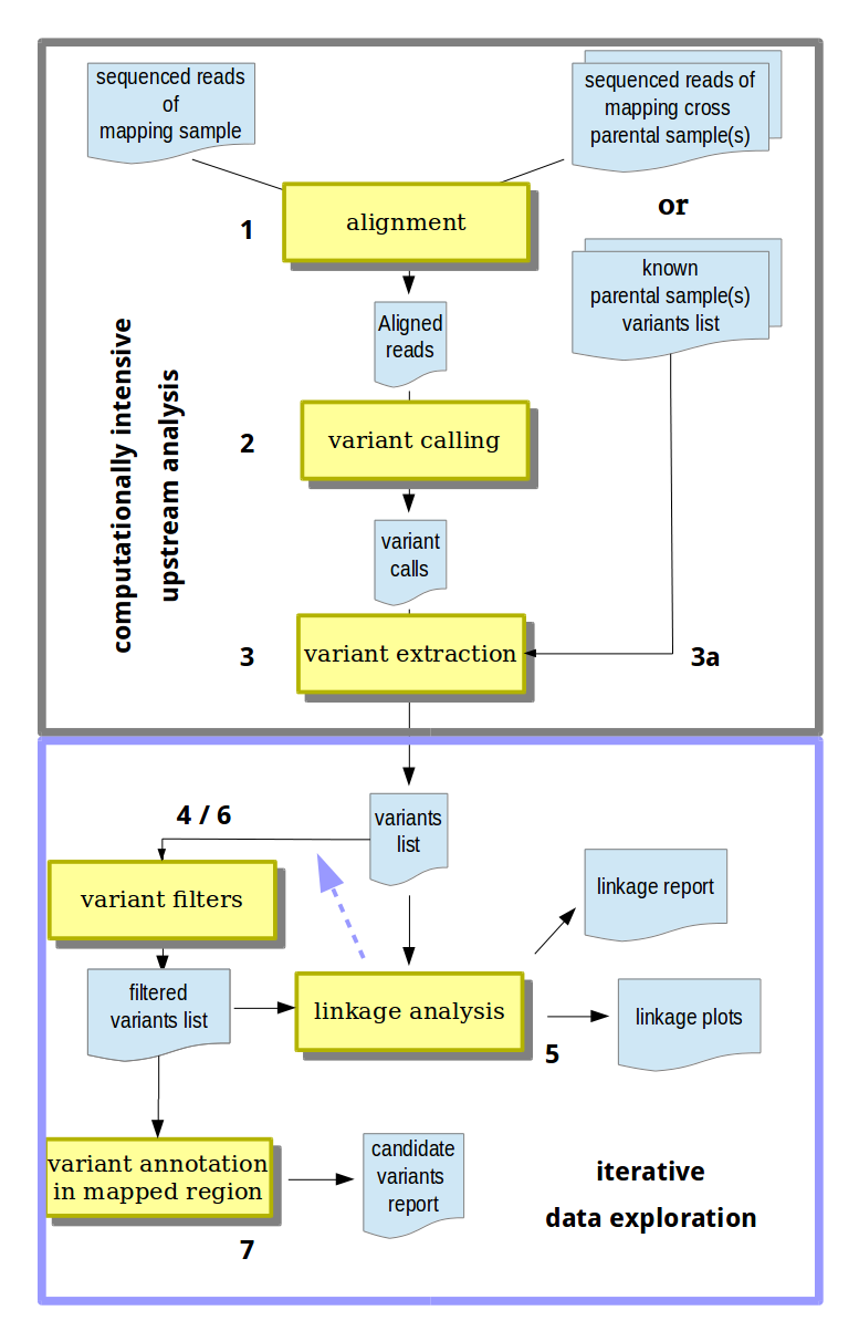
Mapping-by-sequencing analysis workflows in MiModD.
Typically, such an analysis will start with the sequenced reads files of a mapping sample and of one or two parental samples that contributed marker variants to the mapping and the first steps will be to:
Align the sequenced reads of all samples that you are going to use in your analysis to their reference genome. The MiModD snap-batch tool from the command line and the Read Alignment tool from Galaxy are making this step especially convenient since they allow you to align all samples in a single run of the tool and to combine the results into a single output file for use in the next step.
You are free, however, to align the reads of each sample separately and produce one output file per sample, if you prefer, and only combine the data in step 2 below. This can be of advantage if you are planning to reuse the aligned data from one of the samples in several independent analyses like, e.g., if you are using the same mapping strain in several independent mutagenesis screens.
Also note that if you are using a third-party aligner like, bowtie2 or bwa-mem instead of the MiModD-provided tools to align your reads, then separate per-sample alignment jobs will typically be your only option.
Use the resulting aligned reads file(s) and the reference genome as input to the varcall command line or the Variant Calling Galaxy tool to obtain a single bcf file with genome-wide per-nucleotide variant call statistics for all samples.
Remember that joint analysis of several sequencing datasets is one of the strengths of MiModD. If you have sequenced several related samples, you can increase sensitivity in calling variants and gain analysis power in later steps. This is why MiModD is designed around multisample analyses and you should use the aligned reads from all your samples in a single variant call tool run.
Extract bona fide variant sites (in any of the samples) from the bcf file and store them in vcf format using the varextract command line tool or the Extract Variant Sites tool in Galaxy.
3a. At this stage it is possible to merge in independently obtained variant lists for additional samples. See Mapping with known variants for when this can be useful.
At this point, the computationally intensive part of the analysis is completed. While the above steps are long-running tasks that you may want to execute, at least from Galaxy, as an unattended workflow, the remaining steps are fast, but less predictable.
- Variants that cannot be causative based on their cross-sample inheritance pattern (e.g., those present in non-phenotypic samples) or that would misguide the linkage analysis can be eliminated using the vcf-filter tool (Galaxy tool name: VCF Filter).
- Linkage evidence provided by the remaining variants is analyzed and visualized with the map tool (Galaxy tool name: NacreousMap) to pinpoint causative variants to genomic intervals.
- Using this mapping information, the original list of extracted variants from step 3 or 4 can be re-inspected (possibly using the vcf-filter tool again) to identify candidates for the causative variant.
- The resulting list of candidate variants can be annotated to learn about their effects on genomic features like transcripts and genes. Combine the annotate (Galaxy name: Variant Annotation) and varreport (Galaxy name: Report Variants) tools for this purpose.
Hint
Other chapters of this user guide, in particular the Tutorial, explain in detail how to perform steps 1-3 above to identify variants with MiModD and, if you are very new to MiModD, we recommend you to work through them before returning to this section.
The vcf-filter tool required at steps 4 and 6 is introduced in the Multi-sample analysis section of the Tutorial.
For users of the MiModD Galaxy interface, the accompanying example workflow 2 available from the MiModD download site can serve as a template for automating steps 1-4 above through a Galaxy workflow.
The third section of the Tutorial contains an example of linkage analysis as in step 5, but does not explain things in as much detail as we will try in this section.
Variant annotation and reporting (step 7) is illustrated in both the second and the third section of the Tutorial.
Three types of linkage analyses in MiModD
The core tool for linkage analysis in MiModD (step 5 above) is the map tool. It accepts input in VCF format describing variant sites in possibly multiple samples and generated, e.g., by the varextract or vcf-filter tools at steps 3 or 4 above.
Note
The map tool can be used to generate variant linkage reports or plots. For plotting, the tool requires working installations of R and rpy2.
If you want graphical output, but do not want to install additional software, you are encouraged to upload your analysis results to our public NacreousMap server and plot it there.
This tool can be run in either of three modes:
Simple Variant Density (SVD) mapping
In SVD mode the tool generates reports of and/or plots the genome-wide
distribution of ALL variants listed in its input.
To this end it calculates variant density in user-configurable bin widths and scales the per-bin values so that they add up to one across all contigs.
The graphical output is in the form of histograms (one per reference chromosome). The text report contains the histogram data in table form for import into spreadsheet applications or other analysis software.
In this mode, it is the user’s responsibility to pre-filter the variant input list in an appropriate way so that only meaningful variants are passed to the map tool. With the various options provided by the vcf-filter tool this is a powerful and flexible way of visualizing variant linkage patterns following various kinds of mapping protocol.
Variant Allele Frequency (VAF) mapping
VAF mode is more specialized than SVD mode and intended for bulked
segregant analysis, in which data is obtained from a non-uniform (segregating)
population of mapping cross progeny sequenced as a pool. In this mode, the
map tool reports/plots linkage as the relative contribution to
the bulked segregant population of each of two parental alleles at identified
biallelic sites.
Methods Background
When a mutant strain displaying a recessive phenotype of interest is crossed to a divergent mapping strain, then, in a bulk of phenotypic F2 progeny, the relative contribution of each parent allele at biallelic variant sites will provide linkage information. While the bulked segregant population should, on average, inherit alleles from the original mutant background and from the mapping strain with approximately equal likelihood, there should be a marked shift towards inheritance of the original mutant background and exclusion of mapping strain alleles in the vicinity of the selected causative mutation.
In Variant Allele Frequency Mapping, the variants present in the starting strains are not just probed for presence or absence in the mapping cross progeny, but the fraction of variant over reference alleles in the sequenced pool provides a direct estimate of the probability of separating the variant from the phenotype, which is why VAF-type analyses often provide very fine-grained linkage information with relatively little experimental effort.
The disadvantage is that the sequence of at least one of the parental backgrounds has to be known - either from previous work or from sequencing along with the bulked segregant population.
Different from SVD mode, VAF mode requires the VCF input to specify variants from multiple samples:
- one of these samples, obviously, has to be the bulked segregants sample
because it holds the inheritance patterns at all biallelic sites, i.e., the
crucial mapping information.
In MiModD, this sample is referred to as the mapping sample and gets passed
to the map tool through its
-mor--mapping-sampleoption.
The two parental backgrounds, variant information of at least one of which must be provided in the VCF input, play opposite roles in a VAF mapping analysis:
- alleles of the parental background that contributes the mutation to be
mapped, behave similar to how they would in a simple backcrossing scheme.
They will have a higher likelihood to be inherited by any phenotypic F2
individual the closer they are to the mutation of interest.
In MiModD, the sample representing this background is called the related
sample (and gets passed to the map tool via the
-ror--related-sampleoption). - the other parental background is represented by what is called the
unrelated sample in MiModD. It is passed to the map tool through the
-uor--unrelated-sampleoption and inheritance of its alleles is interpreted exactly contrary: low representation in the bulked F2 sample is an indication that the corresponding sites are close to the mutation to be mapped.
The graphical output in VAF mode can, like in SVD mode, take the form of per-chromosome histograms with user-configurable bin widths. These histograms quantify the evidence for linkage to the causative mutation provided by the variants in each bin, i.e., the causative mutation is likely to be found near a peak in the histograms. Like for SVD mode, the text report contains the histogram data in tabular form.
In addition, per-chromosome scatter plots showing allele ratios in the mapping sample at each biallelic variant site can be produced for direct visual identification of regions of linked inheritance. In these plots the y-axis shows observed segregation rate between any variant site and the mutation to be mapped, i.e., the causative mutation is likely to be found in the center of a cluster of data points with y values close to zero. Because with one data point for each biallelic variant site, the scatter plot output becomes crowded easily, a moving average through the y values (more precisely, it is a Loess regression line) can also be plotted and is expected to show a local minimum near the causative variant site.
How linkage evidence is calculated - the technical details
The algorithm used to identify biallelic variant sites and to calculate allele ratios for the mapping sample depends on the type of input you provide for the tool:
If the input contains variants found in all three relevant samples - the mapping, the related and the unrelated sample - and you specify the names of all of them through the corresponding command line options, then the map tool can identify biallelic sites directly. All it does is to look for sites at which the related and unrelated samples are homozygous for different alleles. At such sites it then analyzes the contribution of the two alleles to the mapping sample population and forms the ratio.
If only one of the two parental samples is available, the tool has to guess the allelic constitution of the missing sample.
By default, this will be done by considering only sites, at which the available sample is homozygous for a non-reference allele, and assuming that the missing sample is homozygous for the reference. This will typically be a useful assumption if the two parental backgrounds are not closely related themselves.
Alternatively (with the
-ior--infer-missingoption specified), the tool will look at all sites, at which the provided sample appears to be homozygous for any allele (including the reference allele) and will use the ratio of this allele over any other allele found in the mapping sample data. Obviously that assumption is VERY speculative and only makes sense to use when combined with appropriate pre-filtering of the variant sites using the vcf-filter tool (see the Backcrossed bulked segregants analysis example later in this chapter for a more detailed explanation of the problem and an illustration how to address it).
The ratio of unrelated over related sample allele contribution calculated through any of the above algorithms is what is shown then in the scatterplot output of the tool.
The histogram plots, on the other hand, show a linkage score for variant sites per bin. This score is calulated as the weighed per-bin sum of individual variant linkage scores, which, in turn, are calulated as:
(related parent allele count - unrelated parent allele count)
-------------------------------------------------------------  ^ 3
(related parent allele count + unrelated parent allele count)
The weighing is done based on presumed accuracy of the observed allele ratio expressed as the square root of the sum of parent allele counts. The resulting numbers per bin are normalized to the total number of biallelic sites in the bin and the average linkage evidence provided by the whole corresponding chromosome. The underlying formula used for this normalization is the same as reported in [1], Figure 7. Finally, the bin values get scaled so that they add up to one across all contigs.
Variant Allele Contrast (VAC) mapping
VAC mode compares two samples, a mapping and a contrast sample, at
all sites at which a variant has been called in any sample in the VCF input.
In this mode the tool analyzes the difference in allele composition between the
two samples at all these sites and reports and/or plots the genome-wide
distribution of the divergence between them.
The graphical output is in the form of histograms (one per reference chromosome). The text report contains the histogram data in table form for import into spreadsheet applications or other analysis software.
Since this mode relies on the analysis of allelic ratios at given sites, the quality of the resulting analysis is especially sensitive to coverage at these sites and we recommend you to pre-filter the variant input list for depth-of-coverage so that only sufficiently covered (aim for at least 10x coverage, but more is better) sites are passed to the map tool.
Which mapping mode should I use?
VAF/VAC mode
Simply put, whenever you are analyzing sequencing data from a non-isogenic bulked segregants population, VAF or VAC mode should be your first choice. Even though it is often possible to analyze the same data in SVD mode after careful pre-filtering, the VAF or VAC modes are usually more sensitive at picking up linkage evidence and provide finer mapping.
VAF mode does require variant information from at least two samples - from the bulked segregants population and from at least one of the two parental backgrounds that contributed to its generation. This requirement, however, is less limiting than it may sound at first. For one thing, parental background does not strictly mean that you have to know all the variants present in the parent strains of the mapping cross. Some missing or falsely assumed variants are usually quite tolerable, which means that variant information from a sufficiently related strain will also do. What is more, you can obtain the parental background variants from sequencing the parent or a related strain and analyzing the data along with that of the bulked segregants sample - but you may also use a published variants list (see the info box on Mapping with pre-existing parental variant lists below).
VAC mode, on the other hand, works without any parental marker variant information, but uses a second sample with a supposedly contrasting allele pattern around the causative variant. Ideally, to obtain a maximal contrast between the two samples, this second sample is another F2 pool selected for the opposite phenotype as the mapping sample, but it could also be a non-selected pool or a related strain without any of the marker mutations introduced into the mapping sample.
SVD mode
SVD mode should be used to analyze any mapping approach that is based on the sequencing of individuals or (nearly) isogenic populations. In these situations, you know that you can only have one defined genotype at each variant site and analyzing allele ratios will not provide additional information, but just introduce unnecessary noise.
In addition, SVD mode can be used with only one sample and, generally, in a wider range of applications, for which the map tool does not (yet) provide a specialized mode.
Other views on the three modes
Schneeberger [2] has come up with a classification for mapping-by-sequencing strategies. Sticking to his terminology, you would use VAF mode for the analysis of mutant allele frequency (MAF) mapping experiments, while VAC mode corresponds to what he calls allelic distance mapping. SVD mode, on the other hand, could be used for, but is not limited to, homozygosity mapping.
Users of CloudMap may find it convenient to think of SVD and VAF mode as the analogs of the CloudMap EMS Variant Density and Hawaiian Variant Density Mapping tools, respectively, although the mapping modes in MiModD offer significant improvements over their CloudMap counterparts as explained in the section MiModD for users of CloudMap at the end of this chapter. There is no counterpart of VAC mode offered by CloudMap and no support for this type of mapping strategy.
Hint
Mapping with pre-existing parental variant lists
The simplest way to obtain parent strain variants to work with in VAF mode is to actually sequence and analyze at least one of the parental backgrounds alongside the bulked segregant population. In this case, you can simply combine the sequenced reads obtained from your different samples during the alignment or the variant calling step and tell the map tool about the role (mapping sample, related sample or unrelated sample) of each sample in the linkage analysis. The tool will then automatically detect informative biallelic sites in the multisample variants file produced by variant extraction.
In practice, however, if the mapping strain is (or is closely related to) an established strain in your field with its genomic variants already characterized by others, you may prefer to rely on these previous data instead of resequencing the strain. Often, though, you will not have access to the original sequencing data, but only to published lists of identified variants.
In this common case, you can perform the alignment and variant calling steps just on the data from the bulked segregant sample and include the pre-existing information about variant sites in the parental background at the stage of variant extraction.
To this end, the varextract tool accepts an optional pre-calculated VCF file of variant sites, which it will merge with the variant list extracted from its main called variants input.
This alternative way of including crossing strain information is illustrated
in the MiModD Tutorial section on Incorporating mapping-by-sequencing
strategies and in the Outcrossed bulked segregants analysis section of
the Usage examples below. In addition, you may consult the
varextract tool documentation for more information on
its -p or --pre-vcf option and the expected format of the
pre-calculated VCF file.
Usage examples
Mapping with backcrossed mutant strains
As a typical application that would be analyzed in SVD mode consider a phenotypically defined mutant strain obtained from a mutagenesis screen followed by multiple rounds of backcrossing to the non-mutagenized parent strain.
Although there are typically more powerful strategies, it may be possible to map and identify the causative mutation directly through sequencing the backcrossed strain.
Because of linked inheritance, the phenotypic selection during the backcross will not only have worked on the causative mutation itself, but also on nearby non-causative background mutations introduced during mutagenesis. As a result, the causative mutation, after several rounds of crossing, is expected to be found in the center of a mutation-rich region. This is possible because typical mutagenesis protocols introduce dozens to hundreds of mutations into a genome simultaneously.
To exploit the linkage information, it is essential, of course, to exclude variants from the analysis that exist already in the parent strain and will, thus, be kept during the backcross independently of their distance to the causative mutation. To be able to eliminate these variants, you will have to sequence the non-mutagenized parent strain or, if you have isolated and backcrossed several independent mutant strains from the same mutagenesis screen, sequence all or several of these strains and discard all shared variants as most likely derived from the non-mutagenized parent strain.
Now, let us look at how you might analyze the corresponding sequencing data with MiModD.
Here is your assumed starting material for the variant with one backcrossed strain sequenced together with its parent strain:
ref.fa : fasta format
  the reference genome of your organism

mutant.fw.fq : fastq format
  forward reads from the backcrossed mutant

mutant.rv.fq : fastq format
  reverse reads from the backcrossed mutant

parent.fw.fq : fastq format
  forward reads from the non-mutagenized parent strain

parent.rv.fq : fastq format
  reverse reads from the non-mutagenized parent strain
Step 0 - generate sample metadata for use in the analysis:
# Generate a SAM header for each sample.
# The files are used at the next step to add sample metadata to the
# sequenced reads during the alignment.
# The sample names (specified through the --rg-sm) option is what can
# be used to address a specific sample at later steps.

mimodd header --rg-id 001 --rg-sm bc_mutant --rg-ds "mutant x backcrossed n times to parent strain" -o mutant_hdr.sam
mimodd header --rg-id 002 --rg-sm parent --rg-ds "parent strain of bc_mutant" -o parent_hdr.sam
Step 1 - alignment:
# joint alignment of the bc_mutant and parent sample using paired-end mode for each

mimodd snap-batch -s \
"snap paired ref.fa mutant.fw.fq mutant.rv.fq --iformat fastq --header mutant_hdr.sam -o aligned.bam" \
"snap paired ref.fa parent.fw.fq parent.rv.fq --iformat fastq --header parent_hdr.sam -o aligned.bam"
Step 2 - variant calling:
# combined variant calling for both samples

mimodd varcall ref.fa aligned.bam -o variant_calls.bcf
Step 3 - variant extraction:
# extracting bona fide variants from the binary variant calls file

mimodd varextract variant_calls.bcf -o variants_extracted.vcf
Step 4 - variant filtering:
# Retain only variant sites at which the bc_mutant sample is homozygous mutant
# (genotype 1/1), but at which the parent sample appears to be homozygous wt (0/0),
# i.e., eliminate variants that may have been inherited from the parent strain.

mimodd vcf-filter variants_extracted.vcf --sample bc_mutant parent --gt 1/1 0/0 -o variants_informative.vcf
Step 5 - SVD mapping:
# Generate a plot and a tabular report of the distribution of all variant sites
# that passed the previous step.

mimodd map SVD variants_informative.vcf -o variants_linkage.txt -p variants_linkage.pdf
Step 6 - refiltering variants:
# usually not necessary with just a small number of mutagenesis-induced variants

# We assume that the previous step mapped the causative mutation to
# the interval 4,500,000 - 5,000,000 on chrII.

mimodd vcf-filter variants_informative.vcf --region chrII:4500000-5000000 -o candidates_causative.vcf
And here is a very similar workflow you could use if you had sequenced several independent mutant strains, but not their common parent strain …
Assumed starting material:
ref.fa : fasta format
  the reference genome of your organism

mut1.fw.fq : fastq format
  forward reads from the backcrossed mutant1 sample

mut1.rv.fq : fastq format
  reverse reads from the backcrossed mutant1 sample

mut2.fw.fq : fastq format
  forward reads from the backcrossed mutant2 sample

mut2.rv.fq : fastq format
  reverse reads from the backcrossed mutant2 sample

mut3.fw.fq : fastq format
  forward reads from the backcrossed mutant3 sample

mut3.rv.fq : fastq format
  reverse reads from the backcrossed mutant3 sample
Step 0 - generate sample metadata for use in the analysis:
# Generate a SAM header for each sample.
# The files are used at the next step to add sample metadata to the
# sequenced reads during the alignment.
# The sample names (specified through the --rg-sm) option is what can
# be used to address a specific sample at later steps.

mimodd header --rg-id 001 --rg-sm bc_mutant1 --rg-ds "mutant1 backcrossed n times to parent strain x" -o mut1_hdr.sam
mimodd header --rg-id 002 --rg-sm bc_mutant2 --rg-ds "mutant2 backcrossed n times to parent strain x" -o mut2_hdr.sam
mimodd header --rg-id 003 --rg-sm bc_mutant3 --rg-ds "mutant3 backcrossed n times to parent strain x" -o mut3_hdr.sam
Step 1 - alignment:
# joint alignment of the bc_mutant samples using paired-end mode for each

mimodd snap-batch -s \
"snap paired ref.fa mut1.fw.fq mut1.rv.fq --iformat fastq --header mut1_hdr.sam -o aligned.bam" \
"snap paired ref.fa mut2.fw.fq mut2.rv.fq --iformat fastq --header mut2_hdr.sam -o aligned.bam" \
"snap paired ref.fa mut3.fw.fq mut3.rv.fq --iformat fastq --header mut3_hdr.sam -o aligned.bam"
Step 2 - variant calling:
# combined variant calling for all samples

mimodd varcall ref.fa aligned.bam -o variant_calls.bcf
Step 3 - variant extraction:
# extracting bona fide variants from the binary variant calls file

mimodd varextract variant_calls.bcf -o variants_extracted.vcf
Step 4 - variant filtering:
# Retain only variant sites at which the bc_mutant1 sample is homozygous mutant
# (genotype 1/1), but at which the other samples appear to be homozygous wt (0/0),
# i.e., eliminate variants that may have been co-inherited from the common parent strain.

mimodd vcf-filter variants_extracted.vcf --sample bc_mutant1 bc_mutant2 bc_mutant3 --gt 1/1 0/0 0/0 -o mut1_variants_informative.vcf
Step 5 - SVD mapping:
# Generate a plot and a tabular report of the distribution of all variant sites
# that passed the previous step.

mimodd map SVD mut1_variants_informative.vcf -o mut1_variants_linkage.txt -p mut1_variants_linkage.pdf
Step 6 - refiltering variants:
# usually not necessary with just a small number of mutagenesis-induced variants

# We assume that the previous step mapped the causative mutation to
# the interval 4,500,000 - 5,000,000 on chrII.

mimodd vcf-filter mut1_variants_informative.vcf --region chrII:4500000-5000000 -o mut1_candidates_causative.vcf
The steps above should identify the causative variant in bc_mutant1. Steps 4-6 could then be repeated with the roles of the mutant samples exhchanged to identify the causative mutations in bc_mutant2 and bc_mutant3.
Outcrossed bulked segregants analysis
In the previous example above we had to rely on background mutations introduced along with the causative variant during mutagenesis. Instead of limiting our set of linkage markers to these co-induced variants we could decide to cross the mutant strains (before or after backcrossing) to a more distantly related mapping strain. This would introduce lots of additional markers into the F1 offspring, which, after a round of selfing, would then be segregating in F2 individuals. After sequencing a bulk of F2 progeny selected for the original mutant phenotype you would expect linkage analysis to reveal a region deprived of mapping strain alleles around the causative mutation.
Since the sequenced sample does not represent an isogenic population with defined genotypes at variant sites, but a bulk of segregants you should prefer to use the map tool in VAF mode for the analysis.
The exact analysis workflow depends on whether you have obtained sequencing data also for the mapping strain or whether you want to rely on a published list of variants so two separate examples are provided below, one for each case.
Assuming you have sequenced the mapping strain along with the F2 pool, this is what could be your starting files:
ref.fa : fasta format
  the reference genome of your organism

mutant_F2.fw.fq : fastq format
  forward reads from the F2 segregant pool

mutant_F2.rv.fq : fastq format
  reverse reads from the F2 segregant pool

polymorph.fw.fq : fastq format
  forward reads from the polymorphic mapping strain

polymorph.rv.fq : fastq format
  reverse reads from the polymorphic mapping strain
Step 0 - generate sample metadata for use in the analysis:
# Generate a SAM header for each sample.
# The sample names (specified through the --rg-sm) option is what can
# be used to address a specific sample at later steps.

mimodd header --rg-id 001 --rg-sm F2_pool --rg-ds "mutant F2 pool obtained from outcrossing mutant x to mapping strain y" -o pool_hdr.sam
mimodd header --rg-id 002 --rg-sm mapping_strain --rg-ds "mapping strain used to generate F2_pool" -o polym_hdr.sam

# just to point out that you can combine sample metadata and sequenced reads before the alignment:
# this will produce a BAM file of the unaligned sequenced reads for each sample with the header included.
# When archiving data this should be your preferred format since it protects against loss of sample annotations.

mimodd convert mutant_F2.fw.fq mutant_F2.rv.fq --iformat fastq_pe --oformat bam -h pool_hdr.sam -o mutant_F2.bam
mimodd convert polymorph.fw.fq polymorph.rv.fq --iformat fastq_pe --oformat bam -h polym_hdr.sam -o polymorph.bam
Step 1 - alignment:
# aligning from BAM files with combined and annotated paired-end data

mimodd snap-batch -s \
"snap paired ref.fa mutant_F2.bam --iformat bam -o aligned.bam" \
"snap paired ref.fa polymorph.bam --iformat bam -o aligned.bam"
Step 2 - variant calling:
# combined variant calling for all samples

mimodd varcall ref.fa aligned.bam -o variant_calls.bcf
Step 3 - variant extraction:
# extracting bona fide variants from the binary variant calls file

mimodd varextract variant_calls.bcf -o variants_extracted.vcf
Step 4 - VAF mapping:
# VAF mapping here can be done directly without prior filtering.
# The map tool will only consider variant sites that appear to be homozygous
# mutant in the mapping strain.

mimodd map VAF variants_extracted.vcf -m F2_pool -u mapping_strain -o variants_linkage.txt -p variants_linkage.pdf
Step 5 - filtering variants:
# Post-filtering is essential in this example because the F2_pool data will
# contain a huge number of variants inherited from the mapping strain.
# We eliminate these by asking for variant sites at which the selected F2_pool is homozygous mutant,
# but at which the mapping strain has a wt genotype.

# We assume that the previous step mapped the causative mutation to
# the interval 4,500,000 - 5,000,000 on chrII.

mimodd vcf-filter variants_extracted.vcf --region chrII:4500000-5000000 --sample F2_pool mapping_strain --gt 1/1 0/0 -o candidates_causative.vcf
If you have a variant list of the mapping strain instead of actual sequenced reads …
your starting files may look like these:
ref.fa : fasta format
  the reference genome of your organism

mutant_F2.fw.fq : fastq format
  forward reads from the F2 segregant pool

mutant_F2.rv.fq : fastq format
  reverse reads from the F2 segregant pool

variants_polymorph.vcf : vcf format
  preidentified variants for the polymorphic mapping strain
Step 0 - generate sample metadata for use in the analysis:
# Generate a SAM header for the sequenced sample.

mimodd header --rg-id 001 --rg-sm F2_pool --rg-ds "mutant F2 pool obtained from outcrossing mutant x to mapping strain y" -o pool_hdr.sam

# just to point out that you can combine sample metadata and sequenced reads before the alignment
# recommended for archiving as explained in the previous example

mimodd convert mutant_F2.fw.fq mutant_F2.rv.fq --iformat fastq_pe --oformat bam -h pool_hdr.sam -o mutant_F2.bam
Step 1 - alignment:
# aligning from a single BAM file with combined and annotated paired-end data

mimodd snap paired ref.fa mutant_F2.bam --iformat bam -o aligned.bam
Step 2 - variant calling:
# variant calling
# identical to previous example though there is only one sample this time

mimodd varcall ref.fa aligned.bam -o variant_calls.bcf
Step 3 - variant extraction:
# extract bona fide variants from the binary variant calls file and
# MERGE them WITH THE KNOWN VARIANTS from the mapping strain through use of the --p option.
# If variants_polymorph.vcf provides a sample name, this name can be used to address
# the mapping strain sample at later steps, otherwise the name "external_source_1" will be used.

mimodd varextract variant_calls.bcf -p variants_polymorph.vcf -o variants_extracted.vcf
Step 4 - VAF mapping:
# VAF mapping here can be done directly without prior filtering.
# The map tool will only consider variant sites that appear to be homozygous
# mutant in the mapping strain.

mimodd map VAF variants_extracted.vcf -m F2_pool -u external_source_1 -o variants_linkage.txt -p variants_linkage.pdf
Step 5 - filtering variants:
# Post-filtering is essential in this example because the F2_pool data will
# contain a huge number of variants inherited from the mapping strain.
# We eliminate these by asking for variant sites at which the selected F2_pool is homozygous mutant,
# but at which external_source_1 has a wt genotype.

# We assume that the previous step mapped the causative mutation to
# the interval 4,500,000 - 5,000,000 on chrII.

mimodd vcf-filter variants_extracted.vcf --region chrII:4500000-5000000 --sample F2_pool external_source_1 --gt 1/1 0/0 -o candidates_causative.vcf
Backcrossed bulked segregants analysis
As a combination of the first two examples, you may consider a strategy, in which a mutant obtained from a mutagenesis screen is crossed to the non-mutagenized parent strain just once followed by a round of inbreeding and pooling of phenotypic F2 progeny. Assume further that you obtained sequencing data of the pooled F2 progeny and of the premutagenesis strain.
In this case, the mapping relies on background mutations introduced during mutagenesis as in the first example, but uses a bulked segregants approach as in the second.
The fact that you have sequenced a non-isogenic bulked population serves as an indication that using the map tool in VAF or VAC mode may give better results than an analysis using SVD mode.
In addition, this time, you do not have a parental sample from which the tool could obtain the marker variants directly, but you would rather want to look for a region with variant alleles that is present in the pooled data, but not in the premutagenesis parent sample, i.e., you are looking for a region, in which the allele repertoire of the two samples diverges. This situation is best handled by VAC mode, which should, thus, be your preferred choice for this kind of analysis.
Here are your presumed starting files:
ref.fa : fasta format
  the reference genome of your organism

mutant_F2.fw.fq.gz : gzipped fastq format
  forward reads from the F2 segregant pool

mutant_F2.rv.fq.gz : gzipped fastq format
  reverse reads from the F2 segregant pool

parent.fw.fq.gz: gzipped fastq format
  forward reads from the premutagenesis strain

parent.rv.fq.gz: gzipped fastq format
  reverse reads from the premutagenesis strain
and this is how you may analyze them …
Step 0 - generate sample metadata for use in the analysis:
mimodd header --rg-id 001 --rg-sm F2_pool --rg-ds "mutant F2 pool obtained from outcrossing mutant x to its non-mutagenized parent strain" -o bc_pool_hdr.sam
mimodd header --rg-id 002 --rg-sm parent --rg-ds "non-mutagenized parent strain of mutant x" -o parent_hdr.sam
Step 1 - alignment:
# similar to previous examples
# for a change, we assume the sequenced reads to come from gzip-compressed files

mimodd snap-batch -s \
"snap paired ref.fa mutant_F2.fw.fq.gz mutant_F2.rv.fq.gz --iformat gz --header bc_pool_hdr.sam -o mimodd_aln.bam" \
"snap paired ref.fa parent.rv.fq.gz parent.rv.fq.gz --iformat gz --header parent_hdr.sam -o mimodd_aln.bam"
Step 2 - joint variant calling:
mimodd varcall ref.fa mimodd_aln.bam -o mimodd_calls.bcf
Step 3 - variant extraction:
mimodd varextract mimodd_calls.bcf -o mimodd_extracted_variants.vcf
Step 4 - variant filtering:
# VAC mode relies on comparing ratios of alleles between two samples so to
# avoid error amplification it requires good coverage at all sites it
# analyzes.
# To ensure this, you should always filter your input data to retain only
# well covered variants (10x coverage in each sample is a minimum you should
# aim for).
# For the example, lets assume we can require 15x coverage and still retain
# enough variants for a reasonable analysis.

mimodd vcf-filter mimodd_extracted_variants.vcf -s F2_pool parent --dp 15 15 -o mimodd_BCF2_variants.vcf
Step 5 - VAC mapping:
# The F2_pool sample is the one we want to base our mapping on and we want
# to use the parent sample as the contrast sample.
# The scatter plots produced in VAC mode are still kind of experimental and
# may be more confusing than helpful for end users so, in the example, we
# disable them.

mimodd map VAC mimodd_BCF2_variants.vcf -m F2_pool -c parent -o mimodd_bcf2_linkage.txt -p mimodd_bcf2_linkage.pdf --no-scatter
Step 6: refiltering of variants:
# The F2 pool should be homozygous mutant for the causative mutation,
# which should not be present in the parental background.

# We assume that the previous step mapped the causative mutation to
# the interval 0 - 6,000,000 on chrIII.

mimodd vcf-filter mimodd_extracted_variants.vcf -s F2_pool parent --gt 1/1 0/0 -r chrIII:0-6000000 -o candidate_variants.vcf
MiModD for users of CloudMap
For several years, CloudMap [1] - accessible online via the main Galaxy server at https://usegalaxy.org - has been a popular choice for the analysis of mapping-by-sequencing experiments conducted with model organisms. MiModD borrows several key ideas and, consequently, shows some similarities, with that earlier software, but aims at providing a much improved user experience.
Where CloudMap makes use of Galaxy workflows to combine existing Galaxy tools into a pipeline for WGS reads alignment and variant calling, and only provides custom code for linkage analysis, MiModD is a standalone solution for complete mapping-by-sequencing analyses. As a consequence, MiModD can get designed for efficiency and user-friendliness instead of around the input/output requirements of individual tools.
As for linkage analysis, the map tool was inspired by the CloudMap EMS Variant Density Mapping, Variant Discovery Mapping and Hawaiian Variant Mapping tools. The switch from CloudMap to MiModD for linkage analysis is easy because the map tool generates plots that look very similar to those produced by the CloudMap tools. At the same time though, the map tool represents a complete rewrite of and fixes many bugs and inefficiencies found in the original CloudMap tools, among them:
a more powerful algorithm for allele frequency analyses
The tool enables mutation mapping using markers from two parents simultaneously (effectively, combining the CloudMap Variant Discovery Mapping and Hawaiian Variant Mapping approaches into one).
Hint
MiModD distinguishes between a related and an unrelated parent sample in variant allele frequency mapping with respect to the original background of the causative mutation. In CloudMap, you would analyze the variants contributed by the related parent to the allele pool of a bulked segregants population with the Variant Density Mapping tool, while those inherited from the unrelated parent would be analyzed separately with the Hawaiian Variant Mapping tool. The MiModD map tool, in contrast, lets you analyze both sets of variants together for higher mapping accuracy.
- same control over variant density plots as over allele frequency plots
- generation of small, responsive pdfs (up to 50x smaller than files generated with CloudMap)
- more plotting options (scatterplots in any combination of colors with or without a Loess regression line, any number of bin-widths in histograms)
- true species-independence of all plots
- less unhandled errors and clearer error messages
If you have your data analyzed through a CloudMap-based workflow, you can still
take advantage of these MiModD-specific enhancements to the linkage analysis
step because the MiModD map tool can analyze variants found in
CloudMap-generated VCF files. As the only restriction, you will need to provide
a CloudMap-style sequence dictionary file through the
-s or --seqdict-file option (even if CloudMap itself would not require
such a file for the specific species you are working with).
Hint
If all you want to use MiModD for is for generating linkage plots, you may be interested in doing so on our public NacreousMap plotting server, instead of installing MiModD on your local system.
If, conversely, you want to use MiModD for the upstream analysis of your WGS
data, but to use CloudMap for plotting, the map tool lets you
produce CloudMap-ready VCF-like files by combining its --cloudmap and
-t or --text-file options.
| [1] | (1, 2) Minevich et al. (2012): CloudMap: A Cloud-Based Pipeline for Analysis of Mutant Genome Sequences. Genetics, 192:1249-69. |
| [2] | Schneeberger et al. (2014): Using next-generation sequencing to isolate mutant genes from forward genetic screens. Nature Reviews Genetics, 15:662-676. |