First steps: single-sample analysis of a cyanobacteria strain
Background
Synechocystis sp. PCC 6803 is a representative, well-studied strain of Synechocystis, a genus of cyanobacteria. It serves as a model organism for studies on photosynthesis and carbon and nitrogen metabolism. Several substrains with particular phenotypes have been derived from PCC 6803 through cultivation in different laboratories since its original isolation from a freshwater lake in 1968. One of them is the so-called Moscow substrain (PCC-M) which belongs to a subgroup of motile strains as compared to the non-motile substrain from which the PCC 6803 reference sequence was obtained in 1996.
The sequence of the PCC-M strain was reported and compared to that of the PCC 6803 reference in 2012 [1] and in this example we will try to recapitulate that analysis using MiModD.
The PCC6803.tar.gz archive file that you can obtain from the MiModD download site contains two files:
- the PCC 6803 reference sequence in fasta format, including the bacterial chromosome, the four large and two of the three small plasmids of this strain, and
- a BAM file of NGS reads from the PCC-M substrain (the reads are a random subset of those available through the NCBI small reads archive (SRA) under accession number SRX043525).
The goal of this example is to demonstrate the use of MiModD for aligning WGS reads against a reference genome and for discovering sequence variants in the alignment with respect to that reference. In addition, we will have a first look at the variant annotation and data exploration tools of MiModD.
| [1] | (1, 2) Trautmann et al. (2012): Microevolution in Cyanobacteria: Re-sequencing a Motile Substrain of Synechocystis sp. PCC 6803. DNA Res, 19:435-48. |
Step 0: Preparing the data
Data preparation for Galaxy
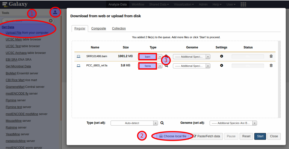
To follow this example analysis using MiModD’s Galaxy interface, you first have to unpack the downloaded dataset archive into a directory of your choice, then upload the reference fasta and the BAM file of WGS reads to Galaxy to make them accessible from the graphical interface. For these relatively small files, the easiest way of doing this is to expand the Get Data section in the Galaxy Tools Bar and select Upload File, or equivalently, click the upload icon at the top of the Tools Bar (1). This pops up Galaxy’s data upload panel, in which you should select Choose local file (2), then select our two input files for upload. Since you know that one of the files is a bam file and that the other one is in fasta format, you can select these types directly (3) instead of letting Galaxy autodetect the formats. Once you have the data upload panel populated like in the screenshot, you can click Start to initiate the data import.
Once the uploads are finished and the files have been added to your currently active history (the right sidebar in the Galaxy window) you can proceed to Step 1.
Note
Uploading the data as described above will store a copy of the files in Galaxy (and use extra disk space on your machine). For a more efficient way of getting data into Galaxy see our recipe for importing large files.
For a general introduction to Galaxy and its terminology, you can check out the Learn Section of the Galaxy documentation.
Data preparation for the command line
Apart from extracting the data files from the downloaded archive no special data preparation is required when working from the command line. Throughout this example, we will assume that you are working from the extracted directory as your current working directory. Hence, if you want to follow this example by simply copying/pasting the command line instructions shown in this section, you should, after unpacking the archive, change to the extracted directory with:
cd tutorial_ex1
To confirm that you are in the right directory, try:
ls
, which should list the two data files plus a readme.txt file.
Step 1: NGS Reads Alignment with the MiModD snap tool
The goal of this step is to determine, for the millions of short unaligned sequences in the input BAM file, their mapping to the reference genome.
To perform an alignment with MiModD in Galaxy, expand the MiModD section of tools in the Tools Bar, then select the SNAP Read Alignment tool ( (1) in the screenshot below). This opens the tool’s input form:
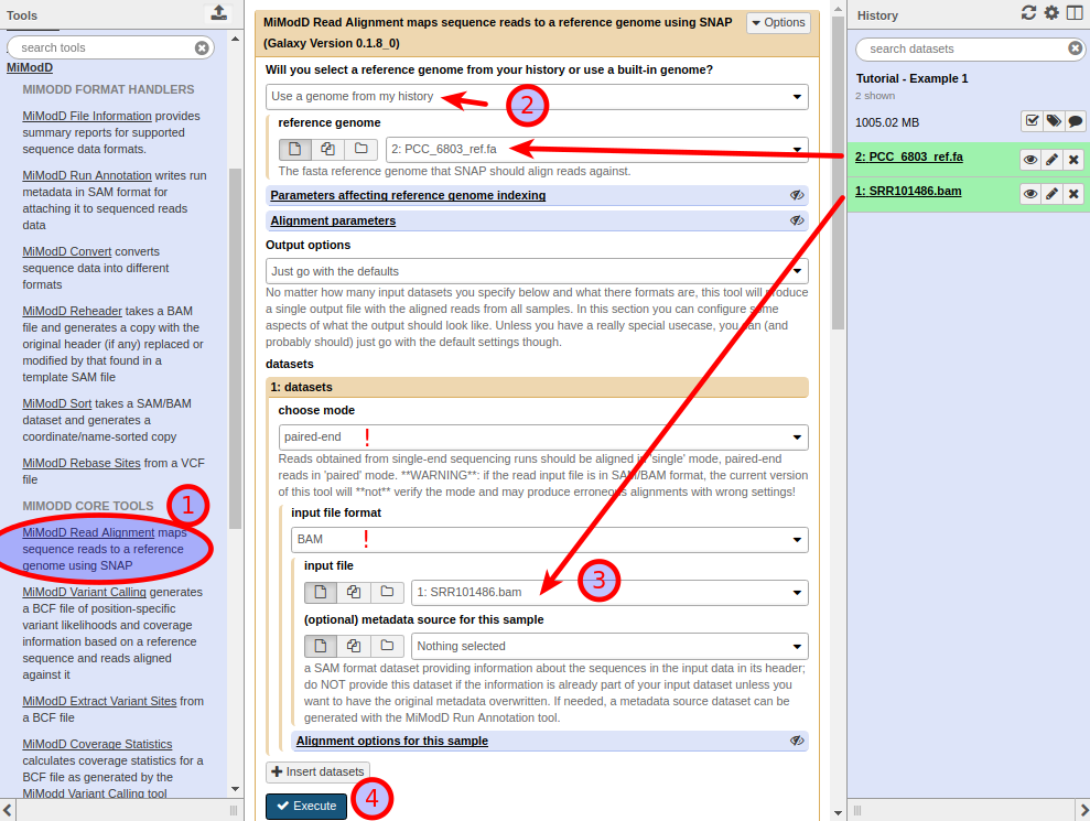
Choose Use a genome from my history from the top-most dropdown menu, then select our fasta dataset as the reference genome (2). Next, under datasets, select the BAM dataset as the input file (3). Note that this will only be possible if the selected input file format is BAM. Since the reads in the example file come from an Illumina paired-end sequencing run, you should also make sure to choose paired-end mode for the dataset.
For this simple example, you can leave all other parameters at their default settings.
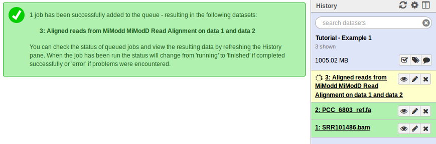
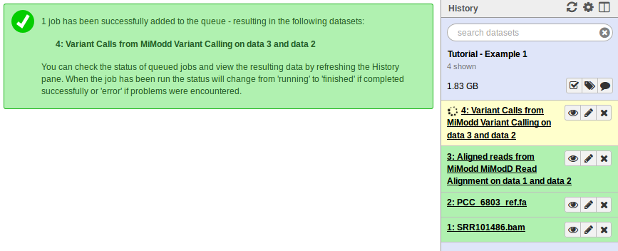
When you click Execute (4) Galaxy will add the new job to your history bar as shown below. Status changes of the job - from scheduled to running to done if all goes well - are indicated by color changes (from grey to yellow to green) of the history item. Depending on your computer’s performance this process should finish within 5 to 15 minutes.
If you are using MiModD from the command line, you can execute the following command to get the exact same result as for the Galaxy job:
mimodd snap paired PCC_6803_ref.fa SRR101486.bam -o SRR101486.aln.bam --verbose
, which will store the alignment of the reads found in the BAM input file against the reference genome in the output file SRR101486.aln.bam.
As explained under Data Preparation, you can simply copy/paste this and the following command line quotes, if you set your current working directory to the directory extracted from the downloaded archive. Otherwise, you will have to add the appropriate paths to all filenames.
Tip
You can get usage information for any MiModD tool from the command line with:
mimodd help <tool name>
so for an overview over all command line options of the snap tool, you can type:
mimodd help snap
, which will tell you that the command can take a host of options, but its general form is:
mimodd snap <sequencing mode> <reference genome> <input file> -o <output file> [OPTIONS]
Here, as throughout the documentation angle brackets < > enclose
parameters to be filled in by the user and square brackets [ ] indicate
optional parameters.
See also
the snap tool description for more details.
Step 2: Identification of Sequence Variants
In the Variant Calling step, each nucleotide in the reference genome gets compared to every overlapping read in the aligned reads file from step 1 to see whether the reference and the sequenced bases agree or whether there is sufficient evidence for a sequence variation at the position.
Below is a snapshot of the Galaxy interface of the MiModD Variant Calling tool:
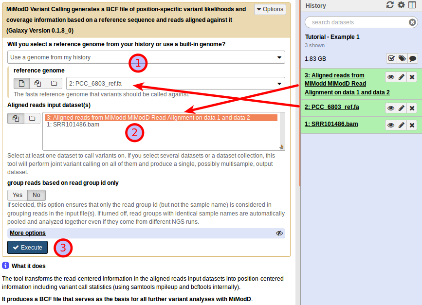
You want to use a genome from your history as the reference genome and make sure your fasta file is selected here again (1). Next, you need to select the dataset with aligned reads you just generated in the previous step as the Aligned reads input dataset (2), and you are ready to execute this job (3). When you do so, another dataset will be added to your history:
This dataset will hold information, for every base in the genome, about
- how many reads in the aligned reads file overlap that base position,
- how many of them agree and disagree with the reference base,
- how well their ensemble supports the reference base or an alternate base instead,
and more. All this per-nucleotide information gets encoded in the binary variant call format BCF to save disk space.
While this means that you cannot view the contents of the file directly in Galaxy (clicking on the dataset’s eye symbol in the history bar will pop up your browser’s download dialog instead), MiModD uses bcf files produced by the Variant Calling tool as a flexible and compact starting point for downstream analyses.
The MiModD command line tool for Variant Calling is varcall and the command line equivalent to the above Galaxy tool run is:
mimodd varcall PCC_6803_ref.fa SRR101486.aln.bam -o example1_calls.bcf --verbose
Tip
MiModD uses general command line options that are understood by several tools in the package.
The -o option (or its long form --ofile) lets you specify the name
of an output file. Without this option, most tools send their output to the
standard output stream, which normally means the screen.
The -v or --verbose option instructs tools to print extra status
messages while they are running.
The -q or --quiet option is recognized by commands that wrap
third-party tools and makes them suppress the original output from these
tools. Be careful with this option though: most of that third-party output
is really informative, when you need to debug a problem or when you are
trying to find the reason for unexpected results. Do not throw away this
information without a reason. One good reason for using the option is if
you want to use a tool in a pipe (and do not worry if you have no idea
what that is again - it is nothing you will have to use to get an analysis
done).
The --quiet and --verbose options can also be combined, though you
will very rarely want to do this. The mimodd varcall command, for example,
uses samtools/bcftools internally for calling variants and --quiet
suppresses any output from these tools, while MiModD itself may produce
--verbose output still.
Step 3: Extraction of variants of interest from the binary variant call file
The principle of variant extraction in MiModD is that you can interrogate a binary variant call file like the one produced in the previous step and, using various filters, retrieve the variants relevant for a specific scientific question in readable form.
The simple question we would like to answer for our example data is:
What genomic variations exist in the sequenced genome of the PCC-M substrain compared to the reference genome ?
and we will use the varextract (Galaxy name: Extract Variant Sites) and vcf-filter (VCF Filter in Galaxy) tools to answer it.
You will, normally, combine these two tools like this to extract variants of interest:
- the varextract tool scans a binary variant call file for positions, at which there is evidence for a variation - this can be a single-nucleotide variant (SNV) or a small insertion/deletion event (indel) - and extracts the information about only these variant positions in vcf format, a human-readable (well, sort of) text format. For typical analyses this extracted variant file still contains many thousands of potential variant sites.
- the vcf-filter tool then lets you specify various filters to apply to an extracted variant file in order to reduce the variants to those meeting your criteria for being relevant and reports them in vcf format again.
In our example, the Extract Variant Sites tool is extremely easy to use:
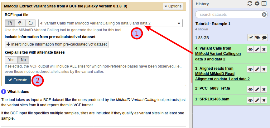
Just select the BCF variant calls file produced in the previous step (1) and start the analysis (2).
Likewise, from the command line simply run:
mimodd varextract example1_calls.bcf -o example1_extracted_variants.vcf
This generates a new dataset, containing per-nucleotide information for only those reference bases that represent predicted variant sites. In contrast to the original binary file, the new file is a text file (in VCF format) that can be inspected directly (by clicking the dataset’s eye symbol in Galaxy):
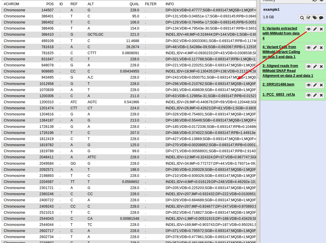
While this gives us a first view on the predicted variants present in our data, the format is clearly not the most user-friendly and with a larger number of variants it quickly becomes impractical to work with so, for data exploration, you would like to:
- reduce the number of variants to consider and
- have better ways of viewing the data.
The vcf-filter tool that we would like to introduce next addresses the first need, while the varreport tool discussed in the next section addresses the second. In general, you will almost always want to filter extracted variants first with vcf-filter before running the varreport tool on the resulting smaller list.
Filtering an extracted variants file
Background
As we have seen above, MiModD reports variant calls in vcf format but, more precisely, it always generates vcf files with genotype columns.
Technically, the vcf format requires 8 tab-separated columns to store general information about its variants, but allows optional columns 9 and higher to hold sample-specific information. MiModD will always produce these so-called genotype columns and most of the filters offered by the vcf-filter tool will work on these columns.
For our example analysis in Galaxy, we want to set up the VCF Filter tool as shown below:
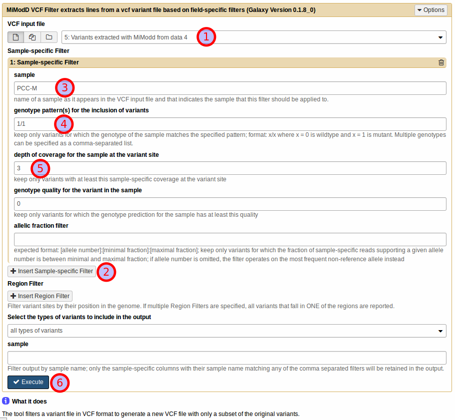
First, select the vcf input file with extracted variants (1).
Then, to define a sample-specific filter, click Insert Sample-specific Filter (2), and, in the expanding section, specify the name of the sample that the filter should work on (3).
The sample name has to match one of the genotype column names in the input vcf file. In our example the name of our only sample was taken from the original BAM file header (see below) and is PCC-M.
Tip
If you are unsure about the sample names or about other general information encoded in any MiModD-supported file type, then without knowing anything about the file format, you can use the info tool (MiModD File Information in Galaxy) to get a standardized summary report.
Next, you need to specify, one or several sample-specific citeria that a given variant in the vcf input will have to fulfill to pass the filter. Currently, the tool lets you define filters based on genotype patterns, depth of coverage, genotype quality, or contribution of specific alleles to the overall number of reads mapped to the site.
Specifying a genotype pattern criterion
Under genotype pattern(s) for the inclusion of variants specify the diploid genotype(s) x/x (with x = 0 for a wt allele, x = 1 for a mutant allele) that should pass the filter.
A variant is retained in the output if the given sample matches one of the specified genotypes for that site.
Note
Variant calling in MiModD assumes a diploid genome. Thus, using MiModD (or, in fact, samtools) for variant calling in haploid organisms may be argued to suffer a conceptual problem but, in practice, results are affected little by this - you just need to decide whether you want to consider the biologically impossible heterozygous genotypes as false calls (as done in this example) or as suboptimally called homozygotes.
For this example, try 1/1 as the genotype pattern for sample PCC-M to retain only variants for which the sample appears to be homozygous mutant (4).
Specifying a depth of coverage criterion
Depth of coverage means the number of reads in your input file(s) of sequenced reads that provided information about the variant site (either favouring the variant or not).
Variants called based on only very few reads are often questionable (since they could easily be caused by sequencing errors), so you can set a lower limit for the read depth here.
For our example, try setting it to three, an often used minimal requirement (5).
Background
depth of coverage here refers to the DP value of the genotype fields, i.e., it is the sample-specific depth of coverage - not to be confused with the overall depth of coverage indicated in the general INFO field of the vcf format.
Specifying a genotype quality criterion
Genotype quality is a score for the reliability of the genotype assignment made by the variant caller. As such, this field may be used to create stricter genotype filters than through the use of genotype patterns alone.
For this example, this criterion can be left at its default value of zero (disabled).
Other filters
The tool also lets you set up two non-sample-specific filters that we will not use in this example. To give a brief description:
- Region filters can be used to restrict the output to variants in certain regions of the genome.
- through the Variant Type filter you can specify whether you want to retain just single-nucleotide variants (SNVs) or only indels.
The sample filter, finally, does not work on rows (= variants), but on the sample-specific genotype columns. It can be used to reduce the number of samples in the output and is supported for compatibility with external tools that may not support multi-sample vcf format. Obviously, this filter cannot be used reasonably on input files with only one sample like our example dataset.
Once you have populated the tool form with all parameters you can execute the job (6), which should finish almost immediately. In general, filtering (and annotating and reporting) variants are very fast processes compared to alignment and variant calling/extraction, making it easy to explore extracted variants quite interactively with many different settings.
To reproduce the Galaxy output from the command line, run:
mimodd vcf-filter example1_extracted_variants.vcf -o example1_filtered_variants.vcf -s PCC-M --gt 1/1 --dp 3 --gq 0
, where the -s or --samples option is, generally, used to specify one
or multiple sample names. For each sample name, a corresponding --gt,
--dp and --gq value needs to be provided, which get then combined in
corresponding order into sample-specific filters (see the vcf-filter tool description for a much more detailed description and
examples of the command line usage of this tool).
By inspecting the filtered output for our example, you can verify that the file format has not changed, but that there are now only 67 variants instead of 78 in the original varextract output. The fact that the filter has not reduced the number of variants more dramatically shows that for this simple dataset with quite high average coverage most variants have been accurately called (see the note on variant calling in haploid genomes above).
Step 4: Generating variant reports
After having narrowed down the list of variants to a manageable length, you will often want to view or print the list in a more human-friendly format than vcf and, with MiModD, this is when the varreport tool (Galaxy tool name: Report Variants) comes into play.
The tool is rather flexible in the kind of reports it can produce, but we are going to use it first in its simplest form, which works with minimal configuration of its parameters.
In Galaxy, simply select MiModD Report Variants and then prepare the tool interface to look like this:
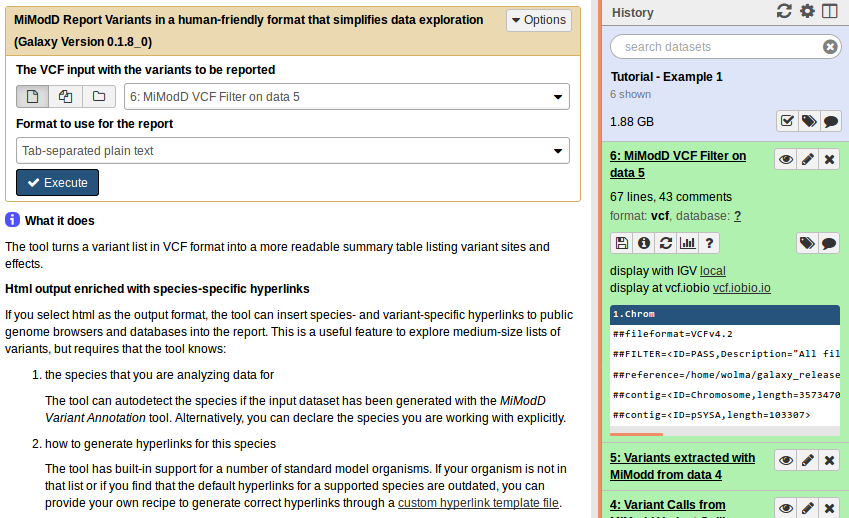
From the command line the equivalent call is:
mimodd varreport example1_filtered_variants.vcf -o example1_variant_report.txt --oformat text
This produces a tab-separated plain text variant report file that should look like this:
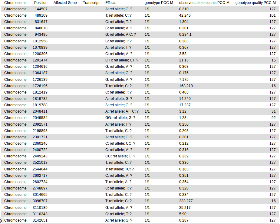
The Affected Gene and Transcript columns are empty in this output because we did not annotate the variants with genomic features they affect. The annotate tool (Galaxy tool name: MiModD Variant Annotation) could be used for this purpose, but we will introduce this tool only in the second example analysis of this tutorial, which will also revisit the generation of variant reports and some of their more powerful features.
In addition, you may consult the detailed varreport and annotate tool descriptions for an explanation of all options available with these tools.
Step 5: Identification of Deletions
Above, you have seen how the combination of the varcall and varextract tools is useful to identify single nucleotide variations (SNVs) and small insertion/deletion events (indels). However, these tools can not detect larger alterations to the genome, like larger deletions and insertions, duplications and translocations. In its current version, MiModD provides only one simple tool to detect deletions in paired-end reads data. Additional tools for the detection of other variations may be added in future releases.
The Deletion Calling (for PE data) tool for Galaxy offers the following interface:
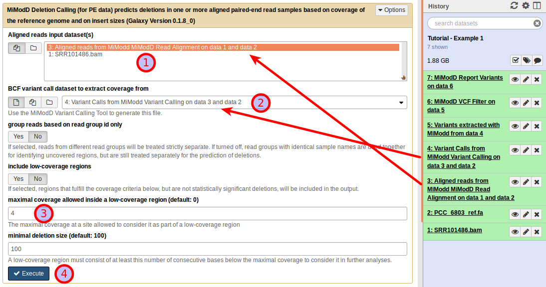
The tool requires two different types of input files:
- an aligned reads file in bam format and
- a bcf file with variant calling information generated from the aligned reads in the first file through the use of the Variant Calling tool.
In our case, we use (1) the aligned reads generated in step 1 and (2) the bcf variant call results generated in step 2.
The tool identifies deletions in a two-step process. First, it looks for low-coverage regions (based on the coverage information stored in its bcf input), then it calculates scores for the likelihood that any low-coverage region is caused by an actual deletion of the genomic region based on the insert size distribution of read pairs flanking it.
There are two parameters to tune the first of these steps: the tool defines a low-coverage region as a contiguous stretch of nucleotides in the reference genome all of which are covered by less than a threshold number of aligned reads. The maximal coverage allowed inside a low-coverage region setting specifies this threshold and the minimal deletion size controls the minimal length for a run of low-coverage nucleotides to be called a low-coverage region. Increasing the first setting and decreasing the second makes the tool consider more regions as candidate deletions that it evaluates in step 2. Doing so increases analysis runtime, but also results in more hits.
There is no generally optimal setting for the maximal coverage parameter. Instead, acceptable settings have to be determined empirically for every dataset. However, for a small genome as in this example that shows very good overall coverage it may be a good idea to increase it over its default value of 0. Specifying a value of 4 will give robust results (3).
For the minimal deletion size, the statistical power of our algorithm relying on insert size distributions decreases with decreasing sizes of the candidate deletions, so setting this parameter to less than its default value of 100 is only advisable with very high overall sequencing coverage. Otherwise, this will just increase the runtime of the tool and produce more uncovered regions, but will not change the number of statistically significant deletions. On the other hand, of course, small deletions may be missed with too restrictive settings. For our example (with quite high coverage) you can compare, if you want to, the result with the default setting of 100 nucleotides to that obtained after reducing the value to 10 nucleotides.
Finally, the output of the tool can be changed by selecting include low-coverage regions . With this option enabled, low-coverage regions that do not pass the statistical test for real deletions will still be included in the output. The resulting list will be much longer than the default output and will contain regions that are poorly covered for technical reasons (e.g., regions refractory to sequencing or regions in which alignment of short reads is problematic). In some cases, the extended list, however, may contain true deletions missed by the algorithm, which may be interesting enough to be followed up by other means. For the example, you can leave the option unchecked, but if you are curious, you may repeat the run with low-coverage regions included, and compare the results.
The group reads based on read group id only checkbox can be left as is for this example.
As always, click Execute (4) to start the job.
Deletion Calling from the command line is done by using the delcall tool. The exact command to reproduce the Galaxy job described above is:
mimodd delcall SRR101486.aln.bam example1_calls.bcf -o example1_deletions.txt --max-cov 4 --min-size 100
End of Part 1 of the Tutorial
At this point, you may wish to compare the result of the analysis with MiModD to the published list of variants [1] for this sample. Do not forget to look at the results of the deletion calling!
This part, however, has only demonstrated the most basic functionality of MiModD for finding variant evidence in WGS data.
In the next section we are going to look at how you can compare variants found in different samples and how that can be helpful to pinpoint variants underlying phenotypes of interest.