Incorporating mapping-by-sequencing strategies: identification of a phenotype-causing mutation in a nematode genome
Background:
Mapping-by-sequencing is a technique that combines classical mapping strategies with genome-wide sequencing. Like for standard mapping procedures, the goal is to determine the position of a mutant allele relative to established markers. However, the power of whole-genome sequencing enables high-precision mapping in one round of mapping crosses and, often, the identification of the mutant allele itself from the same data. Mapping-by-sequencing has been used successfully in most model organisms, including the roundworm Caenorhabditis elegans.
One of the outstanding features of the C. elegans model system is its essentially invariant cell lineage.
As an example, exactly eight out of 959 somatic cells of an adult wild-type hermaphrodite of this nematode species adopt a dopaminergic fate characterized, for example, by expression of the dopamine transporter DAT-1.
From genetic screens, mutant strains could be isolated that show expression of DAT-1 in different numbers of cells than the wild type. One such strain, carrying the recessive mutant allele ot266, shows an aberrantly increased number of dopaminergic neurons in about 9 out of 10 worms [3]. Genome-wide sequencing data involving this mutant has been used as a proof-of-principle dataset for other mapping-by-sequencing pipelines [3], [4].
The references describe, in detail, the generation of the mutant sample that was sequenced. Briefly, mutant animals carrying ot266 were crossed with the Hawaiian CB4856 strain, a classical mapping strain in C. elegans research that shows ~ 100,000 SNVs with respect to the standard lab wild-type strain N2. The resulting F1 progeny was allowed to reproduce by self-fertilization and the resulting F2 progeny was inspected for animals with aberrant DAT-1 expression. 50 phenotypic F2 animals were singled and allowed to reproduce again by self-fertilization. The F3 and F4 progeny were pooled and sequenced using 100-bp reads on an Illumina GA2 sequencer.
The rationale behind this strategy is discussed extensively in the original CloudMap publication [4], but the basic idea is that selection of animals that are homozygous mutant for ot266 results also in selection of nearby N2-specific variants, i.e., in exclusion of Hawaiian CB4856 SNVs in the vicinity of the ot266 allele. From the sequencing data, the molecular change introduced by ot266 can, thus, be identified as a variation that lies in the center of an N2-specific sequence region. The CloudMap pipeline for analysis of mutant genome sequences [4] provides an elegant workflow to identify such N2-specific sequence regions graphically. The dataset is part of the test data accompanying the CloudMap pipeline on the main Galaxy server.
In this section, we will use the ot266 data to demonstrate the usefulness of MiModD in mapping-by-sequencing approaches. In addition, the example will illustrate how straight-forward it is to link the output of MiModD to CloudMap for further analysis.
The worm_ot266.tar.gz archive available as one of the MiModD Project Example Datasets contains these files:
- the C. elegans genome reference sequence in fasta format
- a BAM file of NGS reads of pooled F2 progeny from a cross between an ot266 mutant strain and the Hawaiian mapping strain,
- a BAM file of NGS (Illumina HiSeq 2000 paired-end sequenced) reads from a N2 (wt) laboratory sample (this strain is not the direct parent strain of the ot266 mutant strain, but can serve to correct for errors in the reference genome or artefacts of the alignment step), and
- a Hawaiian strain SNV file in vcf format describing ~ 100,000 SNVs between N2 and the Hawaiian mapping strain with their coordinates matched to the reference genome version.
Except for the N2 control sequence data, these files were taken from the “CloudMap ot266 proof of principle dataset” in the CloudMap section of the public Galaxy Data Library.
| [3] | (1, 2) Doitsidou et al. (2010): C. elegans Mutant Identification with a One-Step Whole-Genome-Sequencing and SNP Mapping Strategy. PLoS One, 5:e15435. |
| [4] | (1, 2, 3) Minevich et al. (2012): CloudMap: A Cloud-Based Pipeline for Analysis of Mutant Genome Sequences. Genetics, 192:1249-69. |
Step 0: Preparing the data
As always, if you are using MiModD through its Galaxy interface, you will have to upload the unpacked files from the downloaded archive to Galaxy.
In addition, we will use this final section of the tutorial to have a first look at sequencing data annotation. While all sequenced reads files in the previous examples were annotated with appropriate metadata describing the sequencing run and the analyzed sample, such information is missing from the N2 sequence file (N2_proof_of_principle.bam). During the different analysis steps in MiModD the software uses these annotations to keep track of individual samples in possibly multi-sample file formats. Since all downstream tools rely on the presence of file metadata, the MiModD alignment tools will not accept sequenced read files as input, if they are not accompanied by metadata!
While SAM/BAM format supports (but does not enforce) a header section for data annotation, fastq format always just stores the sequence information without metadata. Hence, in many cases you will obtain NGS sequencing data first without in-file annotation and you will have to add this information before you can use your data in MiModD. Here, we will introduce the tools to generate annotation metadata with MiModD and to merge them with a BAM file without such information.
Note
For more detailed information about run metadata, SAM/BAM-style headers and how they influence the treatment of multi-sample files by MiModD, we recommend you to read the description of the header tool in the Tool Documentation.
You may prefer to add header information to files from the command line before importing them into Galaxy. This way, you will only have to import the final set of annotated files, but all necessary tools are available also from the Galaxy interface.
To prepare a minimal header for the N2 sequence file, you can try this on the command line:
mimodd header --rg-id 000 --rg-sm N2 -o N2_header.sam
This will generate a minimal SAM-style header declaring a single read-group id (000) and a corresponding sample name (N2) and save it under the chosen output file name.
To generate a new BAM file that merges this header template file with the contents of the N2 sequence file, use:
mimodd reheader N2_header.sam N2_proof_of_principle.bam -o N2.bam
The output file has the minimal required header information now to proceed with the alignment step.
If you prefer to do the annotation in Galaxy, you can do so by using the Reheader BAM file tool:
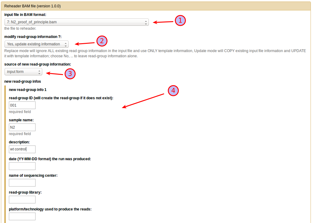
From the input file in BAM format dropdown menu select the original N2 sequenced reads file (1), then choose Yes, update existing information under modify read-group information (2) (in this particular example, since there is no existing information in the file you could just as well select replace existing information instead). This will bring up a further choice of the source of new read-group information, which you will want to set to input form (3). You can then enter the information (make sure you add at least a read-group ID and a sample name) in the text boxes that appear (4). Leave all other selections at their default settings and press Execute.
The dataset that is now generated is the final annotated BAM file that you can use for the further analysis.
See also the reheader tool in the Tool Documentation for a more exhaustive description of options available with this tool.
Step 1: Multi-sample NGS Reads Alignment with the MiModD snap tool
We have looked at this step in detail in the previous Multi-sample Analysis example. In fact, you can proceed exactly as described there, just use the downloaded C. elegans reference sequence and, as sequence input files, the annotated N2 BAM file and the ot266 BAM file.
Make sure you declare the sequencing modes correctly for the two files: choose paired-end for the N2, but single-end for the ot266 data.
If you are working with the command line interface, your command could look like this:
mimodd snap-batch -s "snap paired WS220.64.fa N2.bam -o example3.aln.bam --verbose --quiet" "snap single WS220.64.fa ot266_proof_of_principle.bam -o example3.aln.bam --verbose --quiet"
, which will give you a single results file with the merged alignments of both input files.
Step 2: Identification of Sequence Variants
For variant calling you can proceed exactly as in the first example.
Again, MiModD will correctly identify read groups and samples present in the input file of aligned reads and handle them appropriately.
By now we assume you know how to compose this simple job in Galaxy, but here is the command line equivalent to copy/paste:
mimodd varcall WS220.64.fa example3.aln.bam -o example3_calls.bcf --quiet --verbose
The key to using MiModD in combination with mapping-by-sequencing lies in the next step when variants get extracted from the bcf file: We are analyzing DNA from a pool of F2 animals from a cross of a mutant with a mapping strain and we are interested in the frequency of recombination between any given mapping strain variant and the mutant allele of interest. That is we want to analyze the frequencies at which mapping strain-specific alleles make it into the F2 gene pool. Since this frequency will, actually, be very low in the vicinity of the phenotypically selected mutation, it is not sufficient to extract just the variant sites for which the variant calling step indicates a non-wt genotype. Had we sequenced the mapping strain and analyzed that data together with the F2 pool, the mapping strain variant sites (being homozygous in that strain) would be retained in the output automatically. In our example, however, we do not have original mapping strain sequencing data, but only a downloaded published list of mapping strain variants (as is typically the case for real experiments).
For this case, the varextract tool lets users specify a list of known
variant sites in the form of a pre-calculated vcf file. The HA_SNPs_WS220.vcf
file that is part of this example dataset is such a file and lists about 100000
sites, at which the Hawaiian mapping strain is known to differ from N2. Since
vcf is a plain-text format it is relatively easy to generate a file like this
from any published list of variants. The file can be passed to the varextract
tool through the -p or --pre-vcf option so the command line to extract
the variants of interest from our bcf variant calls file is:
mimodd varextract example3_calls.bcf -p HA_SNPs_WS220.vcf -o example3_extracted_variants.vcf
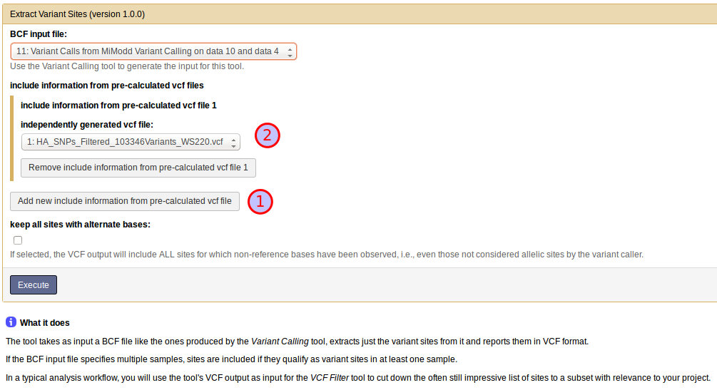
With the Extract Variant Sites tool in Galaxy, you can use the known variants vcf file by clicking on Add new include information from pre-calculated vcf file (1), which will bring up a drop-down menu for the selection of a vcf file (2) as shown below:
Step 3: Data Exploration
You should have a basic understanding of this step already from the previous example.
What we want to retrieve now are variants from the vcf file of all detected variants that appear to be homozygous mutant (genotype criterion 1/1) in the ot266 sample, but homozygous wild-type (0/0) in the N2 sample. Such variants are bona fide candidates for the phenotype-causing mutation.
Try to filter the vcf file produced in the last step with these criteria using either the *vcf-filter* command line tool or the VCF Filter Galaxy tool !
Disappointingly, you will find that this simple filtering technique is by no means efficient enough to give you a manageable list of candidate mutations, e.g. the vcf-filter command line run:
mimodd vcf-filter example3_extracted_variants.vcf -o example3_filtered_variants.vcf -s ot266 N2 --gt 1/1 0/0
yields almost 5000 variants !
Without further tests, it remains unclear whether this large number is due to insufficient coverage of the genome by the relatively small sequenced reads files (which in fact prevents us from using coverage filters along with the genotype criteria above), poor quality of the sequences, alignment artefacts, or actual variant alleles from either the mutagenized strain or the Hawaiian mapping strain that have been inherited by a significant fraction of the pooled F2 animals. What is clear, however, is that we need to combine our simple analysis with some other approach.
This is were mapping-by-sequencing and CloudMap come into play.
Step 4: Data preparation for CloudMap analysis
The Hawaiian Variant Mapping with WGS data tool from the CloudMap series of tools can generate linkage plots from a particular form of a vcf file listing the allele frequency counts for each position in the reference genome that is affected by a known SNV between the N2 and the Hawaiian strain of C. elegans. This information is present in the original extracted variants file generated in step 2, which can be passed to the MiModD cloudmap tool (called Prepare variant data for mapping in the Galaxy interface) to convert it into the format expected by CloudMap.
Note
Despite its name, the CloudMap Hawaiian Variant Mapping Tool can be used for mapping-by-sequencing approaches not just for C. elegans, but any model organism, for which a sequenced mapping strain is available. See the MiModD and CloudMap section of this manual for more information on this topic and on combining MiModD and CloudMap in different kinds of mapping strategies.
Besides the extracted variants file, the tool requires as information:
the desired mapping mode
in VAF - Variant Allele Frequency mode - it produces output ready for CloudMap Hawaiian Mapping, while SVD - Simple Variant Density mode - would give output compatible with CloudMap EMS Variant Density Mapping
the F2 sample (from the extracted variants file) for which mapping should be carried out
the name of at least one parental sample, which provides the variants that should be analyzed for their inheritance pattern in the F2 sample. If the extracted variants file contains variant information for both mapping cross parents, both samples can be specified for simultaneous analysis.
In our example the extracted variants file contains three samples: N2, the ot266 F2 pool, and the pre-calculated Hawaiian strain information. Clearly, the ot266 pool is the sample for which we want to do the mapping and the Hawaiian strain is one of the parental samples that the F2 pool has inherited variants from. In terms of parental samples, the MiModD cloudmap tool distinguishes between related and unrelated samples with respect to the mutant strain. A related parent sample will contribute variants to the F2 pool through the original mutant strain, while an unrelated parent sample will contribute new variants not found in the original mutant strain. The Hawaiian strain, thus, represents an unrelated parent sample.
With this, the command line to generate valid CloudMap input for our example is:
mimodd cloudmap example3_extracted_variants.vcf VAF ot266 -u external_source_1 -o example3_cloudmap_ready.vcf
, where the unrelated parent sample name gets passed through the -u option.
Note
When the varextract tool is used to include information from a pre-calculated vcf file, it will include the samples found in that file as additional ‘virtual’ samples in its output. The autogenerated names of these ‘virtual’ samples will always start with external_source_<file number>, where <file number> indicates from which pre-vcf file the information about the sample was taken (with only one pre-vcf file <file number> will always be 1. If a pre-calculated vcf file specifies its own sample names (not the case in this example), these will be appended to the base name separated through another underscore (_).
As always, you can use the info tool if, at any point, you are unsure about the sample names in a file.
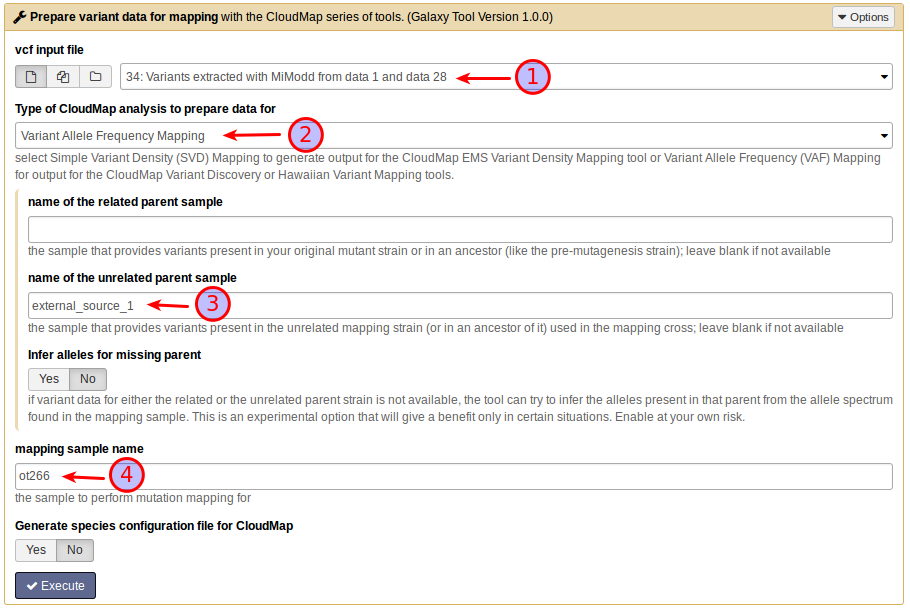
The Galaxy tool interface lets you choose the input file (1) and the analysis mode (2) from drop-down menus and provides text boxes for entering the parental (3) and mapping sample (4) names.
The result file generated by the tool is ready for use with CloudMap as explained in the next step.
The N2 sample has not been used in the above mapping analysis. In principle, the parent sample definitions above allow us to treat the N2 sample as a related parent sample because the ot266 mutant strain, ultimately, has been derived from N2, but, of course, the reference sequence we called variants against is that of N2 as well. Hence, one would expect that any variants called for the N2 sample are either artefacts of the analysis, the consequence of sequencing errors in the reference genome or due to actual differences between N2 laboratory stocks.
Running:
mimodd vcf-filter example3_extracted_variants.vcf -o example3_filtered_N2_variants.vcf -s N2 --gt 1/1
we can quickly check that there are some 3300 variants of this type in our data. Compared to the ~ 100,000 Hawaiian strain variants this is a pretty small number, so including these sites in the mapping analysis is not expected to have a big impact. In other experiments, in which the number of variants contributed by related and unrelated parents is more similar, however, inclusion of both variant sets may make quite a difference. The MiModD cloudmap tool makes it extremely easy to do this combined analysis. In our example we can simply run:
mimodd cloudmap example3_extracted_variants.vcf VAF ot266 -r N2 -u external_source_1 -o example3_cloudmap_ready_with_N2.vcf
, where the only difference to our previous analysis is that we included the N2
sample as related parent through the -r option. If you want to compare the
two results just analyze this new output file as described below for the first
result file.
Note
Though not used in this example, the MiModD cloudmap tool can also generate the species configuration file required by CloudMap for species other than C. elegans and A. thaliana.
With parent samples declared as related or unrelated, MiModD will automatically interpret and format allele frequencies correctly.
The original CloudMap pipeline distinguishes mappings relying on related parent variants and unrelated parent variants with the first type getting analyzed separately with the Variant Discovery Mapping tool. The possibility to perform both types of analyses consistently or even combined is one of the major enhancements that MiModD provides and there should be no need to use the Variant Discovery Mapping tool with MiModD-generated data.
See also
- the cloudmap tool description and
- the Mapping-by-Sequencing using MiModD and CloudMap section of this user guide for an in-depth explanation of the use of MiModD upstream of the CloudMap tool suite
Step 5: Mapping-by-Sequencing using CloudMap
Currently, our recommendation for the standard user is to avoid the additional software dependencies introduced by a local installation of CloudMap in favour of using its tools on the central Galaxy server at http://usegalaxy.org . This means that you will have to transfer the cloudmap-compatible vcf file that you just created to that server, but with the small size of typical such files this should not be too much of an inconvenience.
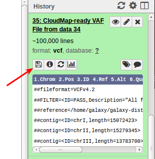
If you have been following this example from Galaxy, you will have to download (i.e. copy) the dataset from your local Galaxy instance to your hard disk before you can upload it to the remote server. To do so, expand the dataset description in the history by clicking on its name, then click on the floppy disk symbol to initiate the download.:
You can upload the file to the remote Galaxy server, by using the Upload File tool just as you would for a local installation.
Once the upload has finished, select the CloudMap: Hawaiian Variant Mapping with WGS data tool, which you can find (at the time of this writing) in the NGS: Variant Analysis section of the Tools bar and configure it as shown below
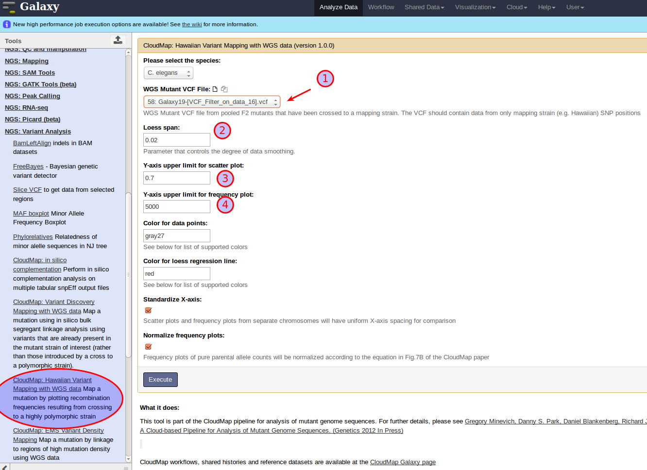
by selecting (1) your uploaded file as the WGS Mutant VCF File. The optimal value to use for the Loess span (2) depends on the accuracy of your mapping data and can only be determined by trying out different settings. In general, with more data points (analysed variant sites) present in the input and with more reliable allele frequency calculations, you should use lower values for the parameter.
Tip
With too small values for a given dataset the tool may fail with a rather cryptic simpleLoess error message about a NA/NaN/Inf in foreign function call. If you see this, just rerun the analysis with a higher Loess span setting.
For controlling the output formatting, you have the option to change the Y-axis upper limit for scatter plot (3) and the Y-axis upper limit for frequency plot (4) as illustrated in the screenshot, but the default values typically work well enough. Click Execute to start the job.
Of the two files that get generated by the tool only the pdf file with a graphical representation of the results is of interest here and you can download it back to your local file system. The figure below summarizes the content of the file:
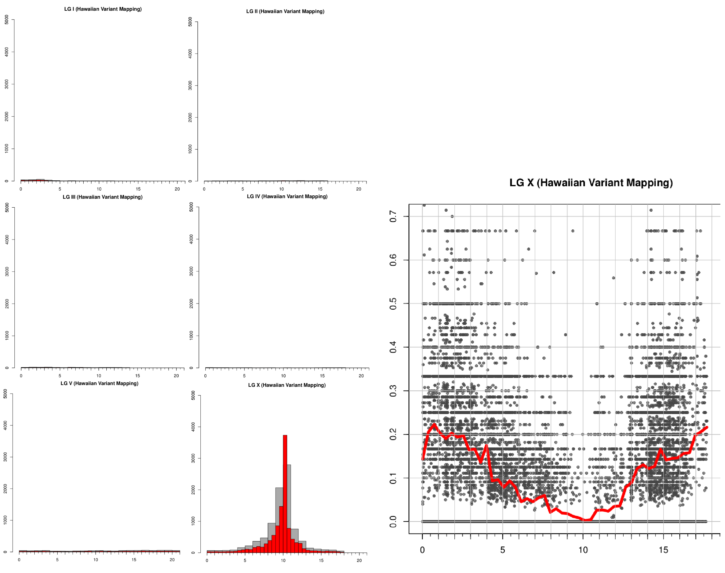
Result generated by the CloudMap Hawaiian Variant Mapping tool.
The histogram plot lets you pinpoint the genomic region linked to the ot266 allele quite convincingly to a small window around 10Mb on Chromosome X !
With this information, we can go back to filtering our variants by their genomic region. We can use the VCF Filter tool once more on the dataset of ~ 5000 SNVs obtained in step 3, either from the command line:
mimodd vcf-filter -r chrX:9000000-11000000 -o example3_peak_variants.vcf example3_filtered_variants.vcf
or from Galaxy by selecting the correct input file, then adding a new Region Filter and defining it as shown below:
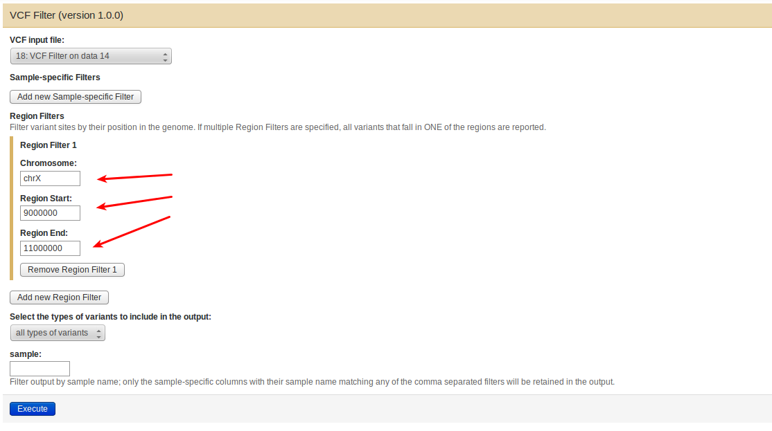
The result of applying the region filter is an encouragingly small file of just 14 SNVs.
As an exercise, you can now try to annotate these variants by using the command line annotate or the Variant Annotation tool in Galaxy to create a report on the filtered variants list with as detailed annotation as you wish !
If you want to generate a fully annotated report with affected transcripts and genes, you will need SnpEff and a suitable SnpEff genome file (see the section on installing SnpEff in this user guide for details). Without SnpEff, MiModD will still be capable of associating genomic positions with the genome browser of the latest Wormbase release. This is done through a built-in species lookup table, so by simply declaring the species as C. elegans when running the annotate tool you can obtain hyperlinks to genome browser views for the positions of all filtered variants.
Warning
It is important to understand that nucleotide numbering may change between different genome versions of the same species. The nucleotide numbers reported in any MiModD output file are determined by the fasta reference sequence you are using in the analysis. SnpEff, on the other hand, uses its own genome files that specify the positions of features in the genome.
To get reliable SnpEff-based annotations it is vital that the fasta reference file and the SnpEff genome file have matching nucleotide numbering. The easiest way to ensure this is to use files with matching refrence sequence version numbers. If that is not possible because SnpEff does not offer a matching genome file, you will have to read through the changelogs of the reference sequence releases for your organism of interest to see if there is an alternative SnpEff genome file version with no nucleotide number changes with respect to your fasta reference.
In the example here, we have used reference sequence version WS220.64 of the C. elegans genome in the upstream analysis so, ideally, we would want a version WS220.64 SnpEff genome file. If you have installed SnpEff version 3.x such a genome file exists, but if you are working with SnpEff 4.x the closest matching available genome file (with no nucleotide number changes) is WBcel215.70.
A similar, though typically less severe issue exists with the linked genome browser views, which are intended to be centered around the respective variant sites. These views are, typically, calculated by the genome browsers based on the nucleotide numbering in the latest reference genome version. If the reference you use in a MiModD analysis is outdated (as it is in this example), the linked view in the genome browser may be shifted. Typically, these shifts will be small and the view will still allow you to see which genomic features exist in the vicinity of candidate variants, but you should not trust them blindly.
A fully annotated report (with the upstream/downstream interval length for SnpEff set to 500 bp) would look like this:
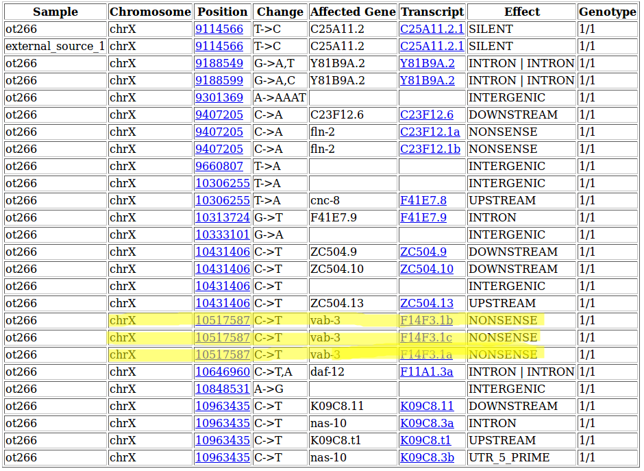
The highlighted SNV at 10,517,587 on Chromosome X represents the known ot266 allele affecting the gene F14F3.1 (also known as vab-3) by introducing a premature Stop-Codon into all of its isoforms. Interestingly, the other nonsense mutation predicted in the region (at 9,407,205) has also been confirmed, but is not responsible for the DAT-1 misexpression phenotype.