Mapping-by-Sequencing with MiModD

Warning

This section still needs an upgrade to reflect the major changes introduced by version 0.1.7 of MiModD.

We are working on it, so check back later ...

What is mapping-by-sequencing

The classical approach to identifying the causative mutation underlying any particular mutant phenotype consists of two separate steps:

• First, genetic mapping is used to narrow down the genomic region that the mutation resides in.

  This is done by introducing defined genetic markers through crossing to a mapping strain and looking for linked inheritance with the mutant phenotype.

• Candidate DNA stretches in that region are then sequenced to identify the mutation.

With whole-genome sequencing it has become possible to merge these two steps into one mapping-by-sequencing step and to speed up mutation identification enormously. After any mapping cross, the inheritance pattern for any set of genetic markers can now be determined along with candidate mutations from the same sequencing data.

Moreover, with mapping-by-sequencing essentially all non-causative mutations (including even previously unknown ones) present in any of the strains used for crossing can be used as marker mutations. This makes mapping-by-sequencing not only a fast, but also an extremely sensitive and versatile method.

To be useful for mapping-by-sequencing experiments, analysis tools need to be able to identify mutations, but also to report or visualize the inheritance pattern of marker mutations so that researchers can use that information to identify the most likely candidate for the causative mutation from the potentially long list of all identified variants.

What is CloudMap ?

CloudMap, accessible through the main Galaxy server at http://usegalaxy.org, is a collection of tools for analysis and visualization of mapping-by-sequencing experiments performed with virtually any model organism. At its core are the three mapping tools:

• CloudMap: EMS Variant Density Mapping,
• CloudMap: Variant Discovery Mapping with WGS data, and
• CloudMap: Hawaiian Variant Mapping with WGS data

, which support the visual interpretation of the marker inheritance patterns obtained from following any of three popular mutation mapping approaches.

More information on CloudMap can be found in the CloudMap online documentation.

MiModD complements CloudMap

CloudMap really facilitates the interpretation of inheritance patterns of sets of mutations. However, the suite itself does not offer tools to identify variants in the first place, but instead, relies on assembling additional tools available on the main Galaxy server into relatively complex workflows.

MiModD makes it possible to perform the complete upstream sequence analysis, generating the input data for the core CloudMap tools, efficiently on a local computer. Hence, it eliminates the need to upload primary sequence data (with huge file sizes) to a remote server.

As a rather specialized package, MiModD also provides a much simpler interface to the necessary alignment, variant calling and variant filtering steps than can be realized by combining standard Galaxy tools.

Finally, MiModD enhances CloudMap by enabling mutation mapping using markers from two parents simultaneously (effectively combining the CloudMap Variant Discovery Mapping and Hawaiian Variant Mapping approaches).

An interface between MiModD and CloudMap

MiModD offers the cloudmap subcommand to transform standard vcf format variant lists generated by the package into valid input for the CloudMap EMS Variant Density Mapping or the Hawaiian Variant Mapping tool.

The CloudMap-compatible output files (typically, these are small enough to be transferred to remote machines conveniently) can be uploaded to the main Galaxy server, or to any other server with the CloudMap tools installed, and be used directly with the corresponding CloudMap tool.

Analyzing whole-genome sequencing data from mapping experiments

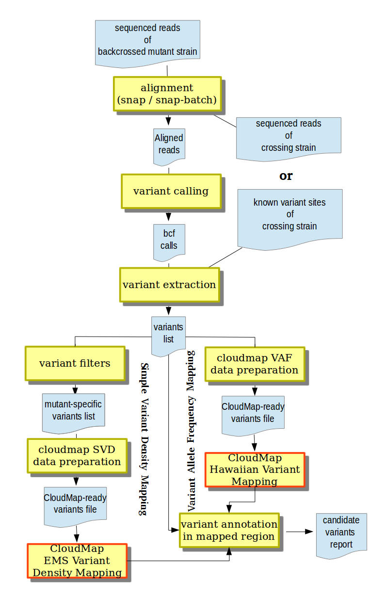
Supported mapping-by-sequencing analysis workflows in MiModD.

Red borders indicate steps that require external CloudMap core tools.

In this section, we review the different strategies for mapping-by-sequencing that CloudMap is compatible with and explain how the corresponding data can be analyzed in MiModD. The figure to the right gives an overview of the general analysis workflows involved.

We assume that you are already familiar with the relevant MiModD tools.

Simple Variant Density (SVD) Mapping

referred to in CloudMap as EMS Variant Density Mapping

In this simple form of mapping, a phenotypically defined mutant strain obtained, for example, from a mutagenesis screen gets backcrossed (selecting for the phenotype) to its non-mutagenized parent strain or outcrossed to a different strain, then sequenced.

Because of linked inheritance, the phenotypic selection will not only work on the causative mutation itself, but also on nearby non-causative background mutations introduced, for example, during mutagenesis. As a result, the causative mutation, after several rounds of crossing, is expected to be found in the center of a mutation-rich region.

This approach works best if the sequence of the crossing strain (parent strain or unrelated) is analyzed along with that of the outcrossed mutant or if several mutants derived from the same parent are analyzed together since this makes it possible to eliminate variants that were not present in the mutant strain, but represent (misinformative) sequence deviations between the reference genome and the crossing strain.

SVD Mapping with MiModD

In most cases, a SVD Mapping analysis will start from at least two datasets of sequenced reads - one from the backcrossed mutant strain and one from the crossing strain. Since the joint analysis of several sequencing datasets is one of the hallmark features of MiModD the subsequent steps (see also the figure above) are straightforward:

1. Align the sequenced reads from both samples to a common reference genome using the snap-batch tool from the command line or the Snap Read Alignment tool from Galaxy.
2. Use the resulting aligned reads file and the reference genome as input to the varcall command line or the Variant Calling Galaxy tool to obtain a bcf file of all observed nucleotide differences between aligned reads and reference sequence.
3. Extract bona fide variant sites (in any of the samples) from the bcf file and store them in vcf format using the varextract command line tool or the Extract Variant Sites tool in Galaxy.
4. Filter the extracted variants for those found ONLY in the backcrossed mutant sample, but not in the crossing strain using the genotype filter of the vcf-filter (VCF Filter in Galaxy) tool. At this step, you will have the choice between filtering for variants for which the mutant sample appears to be homozygous or heterozygous and will have the option to combine the genotype filter with other criteria.

Tip

The Multi-sample analysis section of the Tutorial provides a detailed illustration of all of the above steps.

For users of the MiModD Galaxy interface, the accompanying example workflow 2 available from the MiModD download site can serve as a template for automating this type of analysis through a Galaxy workflow.

Finally, you can pass the resulting filtered vcf file of retained variants to the MiModD map tool (the corresponding Galaxy tool is called Prepare variant data for mapping) specifying SVD (Simple Variant Density Mapping in Galaxy) and the sample name for the mutant strain.

The output produced is ready for use with the EMS Variant Density Mapping tool of CloudMap to visualize clusters of retained mutagenesis-induced sequence variations !

Alternative approach using known crossing strain variants

In practice, if the crossing strain is an established strain in your field with its genomic variants already characterized by others, you may prefer to rely on these previous data instead of resequencing the strain. Often, however, you will not have access to the original sequencing data, but only to published lists of identified variants.

In this common case, you can perform steps 1 and 2 above with just the backcrossed mutant sample, then include the pre-existing information about variant sites in the crossing strain at the stage of variant extraction. To this end, the varextract tool (in step 3 above) accepts an optional pre-calculated vcf file of variant sites, which it will merge with the variant list extracted from its main bcf input.

In the resulting vcf file, the crossing strain will have a genotype of ./. at positions at which it is NOT known to carry a variant and which can be used with the vcf-filter tool in step 4 to retain only variant sites not introduced during the crossing, but pre-existing in the mutant strain.

This alternative way of including crossing strain information is illustrated in the MiModD Tutorial section on Incorporating mapping-by-sequencing strategies. In addition, you may consult the varextract tool documentation for more information on its --pre-vcf option and the expected format of the pre-calculated vcf file.

Variant Allele Frequency (VAF) Mapping

CloudMap distinguishes two flavors of this strategy referred to as Variant Discovery Mapping and Hawaiian Variant Mapping

The underlying approach is an extension of the Simple Variant Density Mapping above.

Instead of generating a single outcrossed strain through several rounds of crossing, the mutant strain, here, gets crossed to the parent strain (or any suitable unrelated strain) only once. Then, the non-uniform (segregating) F2 generation is screened for phenotypically mutant individuals, which are sequenced as a pool, an approach also referred to as bulk segregant analysis. Compared to SVD Mapping, Variant Allele Frequency Mapping provides finer-grained linkage information at less experimental effort since every variant present in the starting strain is not only probed simply for presence or absence after the outcross, but the fraction of variant over reference alleles in the sequenced pool provides a direct estimate of the probability of separating the variant from the phenotype.

As another difference to SVD mapping, variants present in the mutant starting strain and crossing strain variants can be informative in VAF mapping.

VAF Mapping with MiModD

Assuming you have sequenced the F2 pool and the crossing strain, the initial steps of VAF Mapping are identical to those for SVD Mapping (steps 1-3 above). Likewise, if you have to/prefer to use a list of known crossing strain variants instead of actual sequenced reads data for that strain, you can follow the alternative approach using known variants discussed above.

Unlike for SVD Mapping, the vcf-filter tool cannot be used reasonably in VAF Mapping though because applying a genotype filter to a pooled sample of genotypically different individuals does not make sense, neither conceptually nor practically.

Instead, you should pass the multisample variants file obtained from the varextract tool in step 3 to the MiModD map tool unfiltered. Just select VAF/Variant Allele Frequency Mapping mode and indicate the samples representing the pool and the crossing strain, respectively, and the tool will take care of the between-sample comparisons and will produce CloudMap-ready output.

This approach (called Hawaiian Variant Mapping in CloudMap) will map the mutation of interest by analyzing the frequencies with which crossing strain variants are inherited by the F2 progeny. It is illustrated in detail in the third tutorial example on Incorporating mapping-by-sequencing strategies.

Of course, the opposite approach - analyzing the frequencies with which variants from the mutant starting strain are inherited - is also possible. This is called Variant Density Mapping in CloudMap and requires an exactly opposite interpretation of the frequencies since in the vicinity of the mutation of interest the frequency of inheritance of crossing strain variants is expected to drop, while that of mutant starting strain variants should rise.

Unlike CloudMap, MiModD does not treat the two approaches separately, but instead distinguishes between a related and an unrelated parent sample with respect to the original mutant strain. A related parent shares variants with the original mutant strain by descent or, in fact, may be the original mutant strain, and the same definition applies to an unrelated parent sample and the crossing strain. Hence, variants found in the related parent are those that would be analyzed in the Variant Density Mapping-like approach, while the unrelated parent variants are those that the F2 pool may inherit from the crossing strain and that a Hawaiian Variant Mapping-like approach would look at.

You can specify a related parent sample, an unrelated parent sample, or both when running the MiModD map tool (using the command line options --related-parent and --unrelated-parent or the corresponding input fields in the Galaxy tool interface) and the tool will use your assignment to normalize the F2 frequencies for the related parent variants so that they can be interpreted like those of crossing strain variants. In other words, the tool can perform a joint analysis of variants inherited from the mutant strain and the crossing strain, or an analysis of just one of the two classes, but will always produce output for use with the Hawaiian Variant Mapping tool in CloudMap provided you assign the roles of related and unrelated parent sample correctly.