Mapping-by-sequencing: identification of a phenotype-causing mutation in a nematode genome

Background

Mapping-by-sequencing is a technique that combines classical mapping strategies with genome-wide sequencing. Like for standard mapping procedures, the goal is to determine the position of a mutant allele relative to established markers. However, the power of whole-genome sequencing enables high-precision mapping in one round of mapping crosses and, often, the identification of the mutant allele itself from the same data. Mapping-by-sequencing has been used successfully in most model organisms, including the roundworm Caenorhabditis elegans.

One of the outstanding features of the C. elegans model system is its essentially invariant cell lineage.

As an example, exactly eight out of 959 somatic cells of an adult wild-type hermaphrodite of this nematode species adopt a dopaminergic fate characterized, for example, by expression of the dopamine transporter DAT-1.

From genetic screens, mutant strains could be isolated that show expression of DAT-1 in different numbers of cells than the wild type. One such strain, carrying the recessive mutant allele ot266, shows an aberrantly increased number of dopaminergic neurons in about 9 out of 10 worms [3]. Genome-wide sequencing data involving this mutant has been used as a proof-of-principle dataset for other mapping-by-sequencing pipelines [3] [4].

The references describe, in detail, the generation of the mutant sample that was sequenced. Briefly, mutant animals carrying ot266 were crossed with the Hawaiian CB4856 strain, a classical mapping strain in C. elegans research that shows ~ 100,000 SNVs with respect to the standard lab wild-type strain N2. The F1 progeny was allowed to reproduce by self-fertilization and the resulting F2 progeny was inspected for animals with aberrant DAT-1 expression. 50 phenotypic F2 animals were singled and allowed to reproduce again by self-fertilization. The F3 and F4 progeny were pooled and sequenced using 100-bp reads on an Illumina GA2 sequencer.

The rationale behind this strategy is discussed extensively in the original CloudMap publication [4], but the basic idea is that selection of animals that are homozygous mutant for ot266 results also in selection of nearby N2-specific variants, i.e., in exclusion of Hawaiian CB4856 SNVs in the vicinity of the ot266 allele. From the sequencing data, the molecular change introduced by ot266 can, thus, be identified as a variation that lies in the center of an N2-specific sequence region. At the time of its publication, the CloudMap pipeline for analysis of mutant genome sequences [4] provided a remarkably elegant workflow to identify such N2-specific sequence regions graphically.

The dataset that we are going to use in this section is part of the test data that accompanied the CloudMap pipeline on the main Galaxy server. We will use the ot266 data to demonstrate the usefulness of MiModD in mapping-by-sequencing approaches. Users with previous CloudMap experience will recognize the similarity of the results and their visualization with what is produced by the CloudMap Hawaiian Variant Mapping tool, but also the many improvements that MiModD offers over this older tool.

The worm_ot266.tar.gz archive available as one of the MiModD Project Example Datasets contains these files:

• the C. elegans genome reference sequence in fasta format
• a BAM file of NGS reads of pooled F2 progeny from a cross between an *ot266* mutant strain and the Hawaiian mapping strain,
• a BAM file of NGS (Illumina HiSeq 2000 paired-end sequenced) reads from a N2 (wt) laboratory sample (this strain is not the direct parent strain of the ot266 mutant strain, but can serve to correct for errors in the reference genome or artefacts of the alignment step), and
• a Hawaiian strain SNV file in vcf format describing ~ 100,000 SNVs between N2 and the Hawaiian mapping strain with their coordinates matched to the reference genome version.

Except for the N2 control sequence data, these files were taken from the “CloudMap ot266 proof of principle dataset” in the CloudMap section of the public Galaxy Data Library.

[3]	(1, 2) Doitsidou et al. (2010): C. elegans Mutant Identification with a One-Step Whole-Genome-Sequencing and SNP Mapping Strategy. PLoS One, 5:e15435.

[4]	(1, 2, 3) Minevich et al. (2012): CloudMap: A Cloud-Based Pipeline for Analysis of Mutant Genome Sequences. Genetics, 192:1249-69.

Step 0: Preparing the data

As before, if you are using MiModD through its Galaxy interface, you will have to upload the unpacked files from the downloaded archive to Galaxy.

Adding sequencing run metadata

In addition, we will use this final section of the tutorial to have a first look at sequencing data annotation. In the previous examples, all sequenced reads files were already annotated with appropriate metadata describing the sequencing run and the analyzed sample. This time, however, such information is missing from the N2_proof_of_principle.bam file.

Background

The two most important elements to describe a WGS dataset are a unique identifier, called read group ID, for a group of sequenced reads obtained in the same sequencing run, and a sample name identifying the biological sample from which the data was obtained.

Since MiModD relies heavily on the presence of read group and sample metadata to keep track of individual samples through multisample analyses, the MiModD alignment tools will not accept sequenced read files as input, if they are not accompanied by metadata specifying at least a read group ID and a sample name!

While SAM/BAM format supports (but does not enforce) a header section for data annotation, fastq format always just stores the sequence information without metadata. Hence, in many cases you will obtain NGS sequencing data first without in-file annotation and you will have to add this information before you can use your data in MiModD.

MiModD offers three principal ways to add metadata to your WGS data:

1. If you have your data stored in fastq format, our recommended solution is to convert the data to BAM format using the convert tool (Galaxy tool name: MiModD Convert), which lets you add the metadata as part of the conversion.

2. If your data is stored in SAM or BAM format already, but is missing required metadata, you can use the reheader tool (Galaxy name: MiModD Reheader) to generate a copy of your data with the metadata added.

   As implied by its name, this tool can also be used to change existing metadata.

3. For all supported input formats (fastq, SAM, BAM), you can specify missing metadata directly at the alignment step (use the --header option of the snap tool or the corresponding (optional) metadata source parameter offered for each input dataset by the Galaxy Read Alignment tool).

   The snap / snap-batch / Read Alignment tools will then attach the metadata to their aligned reads output directly.

   Note

   Though seemingly convenient, using this way to provide run and sample metadata is discouraged!

   You will be left with input data that still lacks any in-file annotation of its content. In-file metadata is your friend that unambiguously identifies your WGS data and prevents later data mix-up.

   About the only valid use case we recognize for on-the-fly metadata is if your input data really does have its content annotated, but parts of the existing metadata are incompatible with the analysis at hand, e.g., because of name collisions with other input to be used in the same analysis. In this case, the option lets you exchange the problematic parts just for one analysis without creating a potentially confusing copy of your input data.

In this example, the problematic N2 data is in BAM format already and we just need to add the metadata so we go with the second option and use the reheader tool.

When working on the command line, adding the metadata is actually a two-step process, in which you first declare the metadata and store it in SAM format. This so-called SAM header is then used as input for the reheader tool that adds the information to your WGS data.

To prepare a minimal header for the N2 WGS file, you can run:

mimodd header --rg-id 000 --rg-sm N2 -o N2_header.sam

This will generate a minimal SAM header declaring a single read-group id (000) and a corresponding sample name (N2) and save it under the chosen output file name.

See also

For more detailed information about run metadata, SAM/BAM-style headers and how they influence the treatment of multisample files by MiModD, we would like to refer you to the description of the header tool in the Tool Documentation.

To generate a new BAM file that merges this header template file with the contents of the N2 WGS file, use:

mimodd reheader N2_header.sam N2_proof_of_principle.bam -o N2.bam

The N2.bam output file will have the minimal header information required to proceed with the alignment step.

Hint

If you have a little bit of command line experience, you might wonder if it is really necessary to create the intermediate SAM header file. In fact, it is not and you can instead join the two commands in a pipe like this:

mimodd header --rg-id 000 --rg-sm N2 | mimodd reheader - N2_proof_of_principle.bam -o N2.bam

, where the - instructs the reheader tool to read from standard input.

If you prefer to do the annotation in Galaxy, you can do so by using the Reheader BAM file tool:

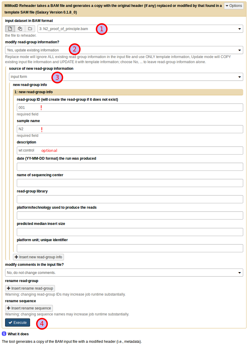
Start by choosing the uploaded N2 dataset as the BAM input dataset (1). Then, under modify read-group information? choose Yes, update existing information (2) (in this particular example with no pre-existing information in the dataset you could just as well select replace existing information instead). This will bring up a further choice of the source of new read-group information, which you should set to input form (3). You can then fill in the text boxes as shown. Note that read group ID and sample name are required fields, while all further information is optional. Finally, leave all other settings at their defaults and press Execute (4) to start the job.

The resulting annotated dataset is ready for use in the alignment step.

See also

the reheader tool in the Tool Documentation for a more exhaustive description of options available with this tool

Step 1: Multi-sample NGS Reads Alignment with the MiModD snap tool

We have looked at this step in detail in the previous Multi-sample Analysis example. In fact, you can proceed exactly as described there, just use the downloaded C. elegans reference sequence and, as sequenced reads input, the freshly annotated N2 BAM file and the ot266 BAM file.

Make sure you declare the sequencing modes correctly for the two files: choose paired-end for the N2, but single-end for the ot266 data.

If you are working with the command line interface, your command could look like this:

mimodd snap-batch -s "snap paired WS220.64.fa N2.bam -o example3.aln.bam --verbose" "snap single WS220.64.fa ot266_proof_of_principle.bam -o example3.aln.bam --verbose"

, which will give you a single results file with the merged alignments of both input files.

Step 2: Identification of Sequence Variants

Calling variants

For variant calling you can proceed exactly as in the first example.

Again, MiModD will correctly identify read groups and samples present in the input file of aligned reads and handle them appropriately.

By now we assume you know how to compose this simple job in Galaxy, but here is its command line equivalent to copy/paste:

mimodd varcall WS220.64.fa example3.aln.bam -o example3_calls.bcf --verbose

Extracting variants

This step introduces one new functionality that is crucial for this example:

We are analyzing DNA from a pool of F2 animals obtained from a cross of a mutant with a mapping strain and we are interested in the frequency of recombination between any given mapping strain variant and the mutant allele of interest. That is, we want to analyze the frequencies at which mapping strain-specific alleles make it into the F2 gene pool. This frequency will, actually, be very low in the vicinity of the phenotypically selected mutation, and it is exactly this low frequency that will be informative for mapping the causative mutation.

However, if we were to extract now just the sites for which the variant calling step indicates a non-wt genotype we would throw away the most informative sites. Had we sequenced the mapping strain and analyzed that data together with the F2 pool, the mapping strain variant sites (being homozygous in that strain) would be retained in the output automatically. In our example, however, we do not have original mapping strain sequencing data, but only a downloaded published list of mapping strain variants (as is often the case for real experiments, too).

In this situation, the varextract tool lets users specify a list of known variant sites in the form of a pre-calculated vcf file. The HA_SNPs_WS220.vcf file that is part of the example dataset is such a file and lists about 100000 sites, at which the Hawaiian mapping strain is known to differ from N2. It can be passed to the varextract tool through the -p or --pre-vcf option so the command line to extract the variants of interest from our bcf variant calls file is:

mimodd varextract example3_calls.bcf -p HA_SNPs_WS220.vcf -o example3_extracted_variants.vcf

Note

Since vcf is a plain-text format it is relatively easy to generate the file expected by the --pre-vcf option from any published list of variants.

With the Extract Variant Sites tool in Galaxy, you can compose your job by selecting the variant call data as the BCF input (1). Next, click on Insert include information from pre-calculated vcf dataset (2), which will allow you to specify the known Hawaiian SNPs dataset as the Independently generated vcf dataset (3).

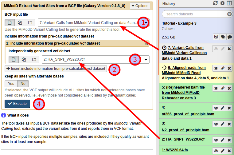
Having the tool interface configured like this, you can press Execute (4) to start the variant extraction.

Step 3: Data Exploration

You should have a basic understanding of this step already from the previous example.

What we want to retrieve this time from the VCF dataset just generated are variants that appear to be

• homozygous mutant in the ot266 sample (genotype criterion 1/1), but
• homozygous wild-type in the N2 sample (genotype 0/0).

Such variants are bona fide candidates for the phenotype-causing mutation.

Exercise

Try to filter the vcf file produced in the last step according to the above criteria using either the vcf-filter command line tool or the VCF Filter tool in Galaxy!

Disappointingly, you will find that this simple filtering technique is by no means efficient enough to give you a manageable list of candidate mutations, but yields almost 5000(!) variants.

Without further tests, it remains unclear whether this large number is due to insufficient coverage of the genome by the relatively small sequenced reads files (which, in fact, prevents us from using coverage filters along with the genotype criteria above), poor quality of the sequences, alignment artefacts, or actual variant alleles from either the mutagenized strain or the Hawaiian mapping strain that have been inherited by a significant fraction of the pooled F2 animals. What is clear, however, is that we need to combine our simple analysis with some other approach.

This is were mapping-by-sequencing and the mimodd map tool (Galaxy tool name: MiModD NacreousMap) come into play.

Step 4: Map a causative mutation through variant linkage analysis

The map tool can generate variant linkage reports and plots from the original variants file obtained in step 2.

Besides the extracted variants file, the tool requires as input:

• the desired mapping mode

  the data in this example is suited for analysis in Variant Allele Frequency (VAF) mode

• the name of the F2 sample (as it appears in the extracted variants file) for which mapping should be carried out

• the name of at least one parental sample, which provides the variants that should be analyzed for their inheritance pattern in the F2 sample. If the extracted variants file contains variant information for both mapping cross parents, both samples can be specified for simultaneous analysis.

See also

The map tool can be used for mapping-by-sequencing approaches not just with C. elegans, but any model organism, and supports a relatively broad spectrum of mapping strategies. For a detailed discussion of concepts and supported mapping approaches see the Mapping-by-Sequencing with MiModD section of this manual.

Assigning roles to samples

In our example the extracted variants file contains three samples:

• the wild type N2 sample,
• the F2 pool selected for the causative ot266 allele by phenotype, and
• the Hawaiian strain represented by its precalculated variant information.

Clearly, the ot266 pool is the sample for which we want to do the mapping and the Hawaiian strain is one of the parental samples that the F2 pool has inherited variants from.

In terms of parental samples, the map tool distinguishes between related and unrelated samples with respect to the mutant strain. A related parent sample is one that contributed variants to the original mutant isolate, and thus to the F2 pool, by descent. An unrelated parent sample, on the other hand, will contribute variants, not found in the original mutant isolate, during the mapping cross. The Hawaiian strain, thus, represents an unrelated parent sample.

See also

An exact definition of the different roles that can be assigned to a sample is provided in the documentation of the VAF mode-specific options of the map tool.

Performing the linkage analysis

Given the above roles of the samples, a valid command line to trigger a variant linkage analysis for our example is:

mimodd map VAF example3_extracted_variants.vcf -m ot266 -u external_source_1 -o example3_linkage_analysis.txt

, where the unrelated Hawaiian strain parent sample name gets passed through the -u or --unrelated-parent option.

Autogenerated external_source sample names

When the varextract tool is used to include information from a pre-calculated vcf file, it will include the samples found in that file as additional ‘virtual’ samples in its output. The autogenerated names of these ‘virtual’ samples will always start with external_source_<file number>, where <file number> indicates from which pre-vcf file the information about the sample was taken from (with only one pre-vcf file <file number> will always be 1). If a pre-calculated vcf file specifies its own sample names (not the case in this example), these will be appended to the base name separated through another underscore (_).

As always, you can use the info / MiModD File Information tool if, at any point, you are unsure about the sample names used in a file.

Using the NacreousMap tool from Galaxy you can compose an equivalent analysis run by populating the tool interface as shown below:

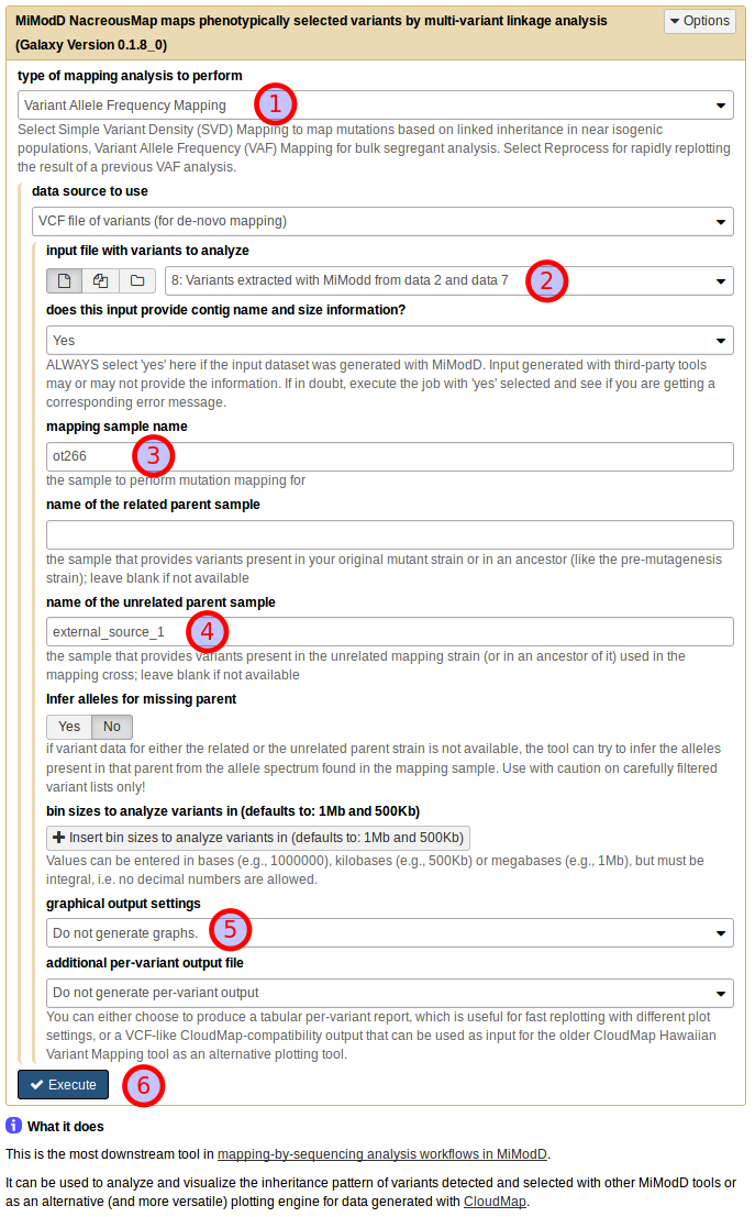
Be sure to select Variant Allele Frequency Mapping as the type of mapping analysis to perform (1) and use the dataset generated by the Extract Variants tool as a VCF file of variants (for de novo mapping) (2). Next, you need to declare the roles that individual samples should play in the linkage analysis (as discussed above): use ot266 as the mapping sample name (3) and external_source_1 as the name of the unrelated parent sample (4). For this first demonstration of the NacreousMap tool, disable its graphical output (5) and start the job (6).

The above simple invocation of the tool produces a single plain-text variant linkage report.

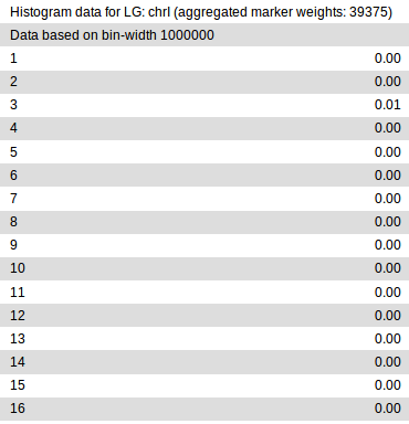
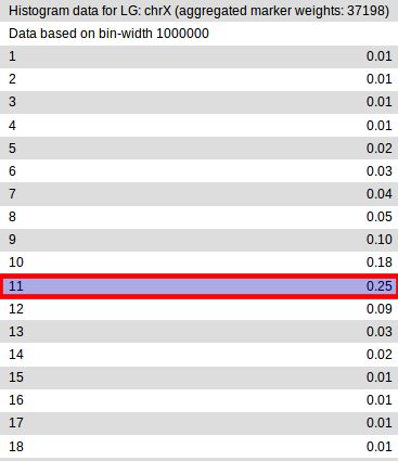
In it, each chromosome defined in the input variant file gets divided into regions of fixed size (bins), in which variants are analyzed separately for evidence of linkage with the mutation of interest. Essentially, the higher the linkage value in a given bin is, the higher is the chance that the mapped mutation resides in that bin. In principle, smaller bin sizes may provide finer mapping, but are also more sensitive to noise and outliers. By default, the results for two different bin sizes (1Mb and 500Kb) are reported (of which only the 1Mb data is shown in the figure). You can specify different bin sizes through the command line -b or --bin-sizes option or in Galaxy under bin sizes to analyze variants in in the NacreousMap tool interface.

>From the partial report shown above, it is clear that in our example, the eleventh 1Mb bin, i.e., the region between 10-11Mb, on chrX has the highest probability of containing the causative variant.

Mapping with two parent samples

You may have noticed that the above linkage analysis did not make use of the N2 sample. In principle, the parent sample definitions above allow us to treat the N2 sample as a related parent sample because the ot266 mutant strain, ultimately, has been derived from N2.

On the other hand, the WS220.64.fa reference genome sequence that we aligned to and called variants against is itself an N2 wild type sequence, so an interesting question is whether our N2 sample has any variants at all then.

Fortunately, this is easy to check by running, e.g.:

mimodd vcf-filter example3_extracted_variants.vcf -o example3_filtered_N2_variants.vcf -s N2 --gt 1/1

, which retains only those variants from all extracted ones, which the variant caller thinks our N2 sample is homozygous mutant for (Galaxy users: try composing the equivalent job using the VCF Filter tool).

The result should tell you that there are approximately 3300 such variants - but how can this be? Here are some possible explanations:

• the variants are sequencing errors or false-positive variant calls, i.e., they do not really exist, neither in the reference genome nor in the analyzed N2 strain,
• it is the reference genome that is wrong at these sites - after all, the reference genome is also the result of sequencing and, thus, may contain sequencing errors - or
• the N2 laboratory stock used in this analysis and the reference N2 that the reference genome got based on really have acquired independent mutations during their lab cultivation history that make them different.

In reality, it is probably a combination of all three effects that we observe here, but it is, conceptually, important to understand that only variants caused by the last effect can help us in the linkge analysis. After all, analysis artefacts, i.e., variants that do not exist in the physical genome, cannot be linked to anything during a cross. If we include these variants as markers in the linkage analysis we will only add noise to the data.

Another aspect is that even though 3300 N2 variants are a surprising lot, they are still a rather small number compared to the ~ 100,000 Hawaiian strain variants that we already used as markers in the single parent analysis so we would not expect that adding them makes a big difference anyway.

The bottom line of all this is that it probably does not make an awful lot of sense to include the N2 sample here as a related parent sample. However, in your own experiments, your mileage may vary: in general, the more diverged from the reference genome you expect your premutagenesis strain to be and the less diverged your mapping strain is from the reference, the more valuable will it be for the linkage analysis to include the premutagenesis strain or a related strain as a related parent. Hence, we think it is worthwhile to demonstrate once how easy it is to carry out a two-parent linkage analysis with the map tool.

In our example we can include the N2 marker variants in the analysis simply by running:

mimodd map VAF example3_extracted_variants.vcf -m ot266 -r N2 -u external_source_1 -o example3_linkage_analysis_with_N2.txt

, where the only difference to the single-parent analysis is that we included the N2 sample as related parent through the -r or --related-parent option.

Galaxy users can simply rerun the previous job, but add N2 as the name of the related parent sample.

The map / NacreousMap tool will then consider marker variants from both parent sides and automatically take into account their opposite meaning for the analysis.

Generating graphical views of the results

The text-based linkage analysis report is often sufficient for mapping a mutation and has the advantage that it can be produced on any system with MiModD installed.

For a graphical view, the report may be imported into third-party software (like Excel), but with just a little bit more effort you can also generate publication-quality plots directly from MiModD. Here you have two options:

• to produce linkage plots on a local system, MiModD requires a working installation of the R statistical analysis software and its Python interface rpy2. The installation instructions section of this user guide offers more information on this topic. With these requirements in place, you can produce pdf-format plots for the above analysis with:

  mimodd map VAF example3_extracted_variants.vcf -m ot266 -u external_source_1 -o example3_linkage_analysis.txt -p example3_linkage_plot.pdf
  

  , which simply specifies an additional (plot) output file through the -p option.

  Likewise, you can then generate an additional plot dataset from Galaxy simply by not disabling the graphical output in the tool interface.

• alternatively, you can also plot pre-processed data on our public mapping-by-sequencing Galaxy server that hosts a stripped-down version of MiModD dedicated exclusively to generating mapping plots. This server-side plot generation offers the same interface and control over tool parameters as the local NacreousMap tool for Galaxy, but by-passes the additional installation requirements.

  If you use the map tool with its -t or --text-file option, like so:

  mimodd map VAF example3_extracted_variants.vcf -m ot266 -u external_source_1 -o example3_linkage_analysis.txt -t example3_variant_report.txt
  

  or, if you ask for an additional Tabular per-variant report in the Galaxy NacreousMap tool,

  

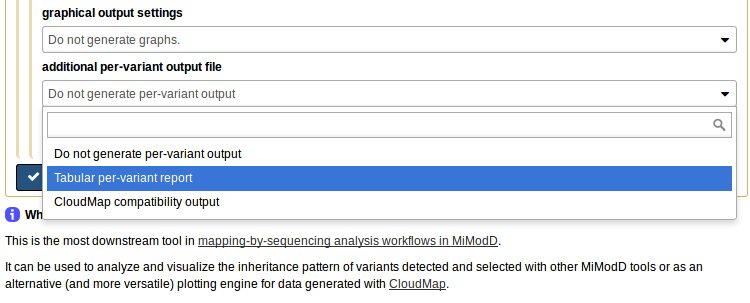
  it produces, as an additional output file, a per-variant report of the map tool analysis, which can be uploaded to our server, or, in fact, any Galaxy server with the NacreousMap tool installed, and be used as compact input to the tool.

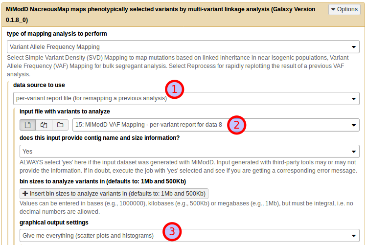
  To make this work, select per-variant report file (for remapping a previous analysis) as the *data source to use (1), then the tabular report you generated on your local system as the input file (2). The report has all the linkage data and the roles of the samples stored in it so you do not have to reassign these anymore. What you still can reconfigure, if you like, is the bin size for analyzing the linkage data and, of course, the plotting options. To use the defaults just choose Give me everything (scatter plots and histograms) under graphical output settings (3) and you are ready to generate your plot on the server.

  

No matter how and where you choose to generate linkage plots, you can configure their exact appearance through a multitude of plotting parameters. These are explained in detail in the plotting options section of the map tool documentation.

Here is an illustration of what you can expect from a linkage plot. Histogram plots for our example data are shown for all six chromosomes of C. elegans. These histograms are the direct visualization of the binned tabular report we looked at before. Of the scatter plots only the one for chrX is shown.

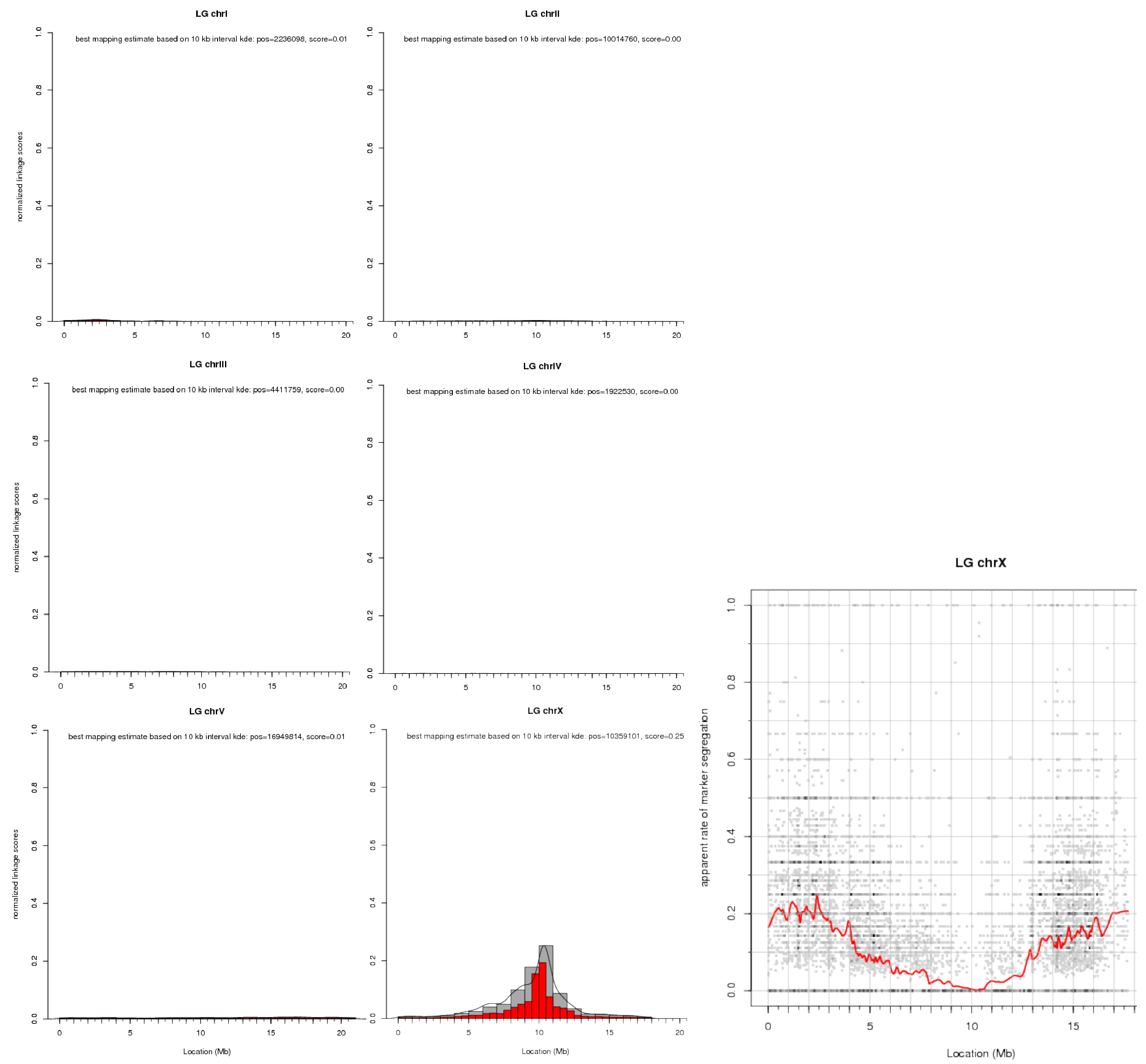
Note that the later shows, for each marker variant, its apparent (based on the input data) rate of segregation from the causative mutation, i.e., the plot shows a dip in the vicinity of the causative mutation.

To prevent scatter plots from becoming too crowded when there is a large number of markers, the tool bins them together and indicates the number of markers in a bin by the color saturation of the corresponding data point. Because there is typically a lot of noise at the individual marker level, a loess regression line through the data is used to show the overall trend in the data.

Step 5: Identify the causative mutation using mapping information

With the information obtained in the previous step, we can go back to filtering our variants by their genomic region. We can use the VCF Filter tool once more on the dataset of ~ 5000 SNVs obtained in step 3, either from the command line:

mimodd vcf-filter -r chrX:9000000-11000000 -o example3_peak_variants.vcf example3_filtered_variants.vcf

or from Galaxy by selecting the correct input file, then adding a new Region Filter and defining it as shown below:

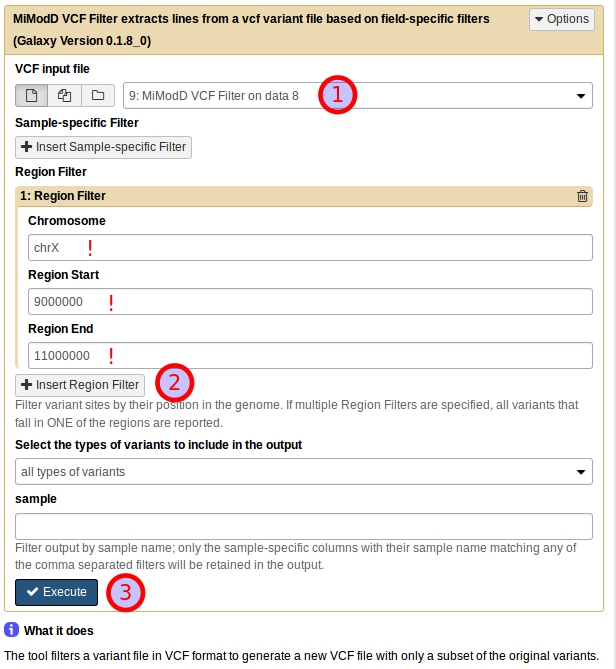
The result of applying this refined filter is an encouragingly small dataset of just 12 variants.

Exercise

Try to annotate these variants using the command line annotate or the Variant Annotation tool in Galaxy, then create a report of the variants and their effects using the command line varreport or the Galaxy Report Variants tool.

We have covered these two tools in detail in the previous chapter.

As before, if you want to generate a fully annotated report with affected transcripts and genes, you will need SnpEff and a suitable SnpEff genome file (see the chapter on installing SnpEff in this documentation for details).

Without SnpEff, MiModD will still be capable of associating genomic positions with the genome browser of the latest Wormbase release. This is done, again, through a built-in species lookup table, so you can profit from this feature if you simply declare the species to be C. elegans when running the annotate tool.

Warning

To get reliable SnpEff-based annotations it is vital that the fasta reference file and the SnpEff genome file have matching nucleotide numbering!

See also

As part of our SnpEff installation instructions we have compiled a section on genome file versions with hopefully helpful suggestions on obtaining coordinate-compatible fasta reference and SnpEff genome files in non-trivial cases.

A similar, though typically less severe issue exists with the linked genome browser views, which are intended to be centered around the respective variant sites. These views are, typically, calculated by the genome browsers based on the nucleotide numbering in the latest reference genome version. If the reference you use in a MiModD analysis is outdated (as it is in this example), the linked view in the genome browser may be shifted. Typically, these shifts will be small and the view will still allow you to see which genomic features exist in the vicinity of candidate variants, but you should not trust them blindly.

In the example here, we have used a fasta reference sequence at version WS220.64 of the C. elegans genome in the upstream analysis so, ideally, we would want a version WS220.64 SnpEff genome file. If you have installed SnpEff version 3.6, such a genome file exists directly. Up to version 4.1, the 4.x series of SnpEff does not have WS220.64 anymore, but offers the fully compatible version WBcel215.70. Since SnpEff 4.2 this is also gone and only subversions of WBcel235 are available, which are coordinate-compatible among each other, but not with WS220.64.

We are bound to the WS220.64 reference because that is the coordinate system that the published Hawaiian strain variants list uses, so our remaining options are:

• install SnpEff v3.6 and configure MiModD to use this version for variant annotation;

  if you already have a newer version installed, you can have v3.6 installed in parallel, then switch MiModD to use this version just for this analysis,

• install SnpEff v4.0 or v4.1 and genome file WBcel215.70, or

• use SnpEff v4.2 or v4.3 (the latest version at the time of writing this) and a WBcel235 genome file, and migrate your candidate variants list to this reference coordinate system before the annotation.

Because it is most instructive (and also because it avoids the above-mentioned genome browser view issue) we are going to show you that third approach.

First, we need the correct chain file to map from WS220 to WBcel235. Navigating our way through the UCSC download page (-> Nematodes -> C. elegans) we get to the C. elegans genome downloads and find that the latest genome version offered for download is WS220/ce10 (where ce10 is the UCSC version identifier, which only gets increased when a reference genome release features coordinate changes). Following on to LiftOver files and scrolling to the bottom of that page, we find a ce10ToCe11.over.chain.gz file. From the list of UCSC genome releases we can learn that ce11 corresponds to the coordinate system used in WBcel235 and later so this chain file is what we are looking for.

Now to rebase the coordinates from this example, download this file into your current working directory and run the rebase tool with:

mimodd rebase example3_peak_variants.vcf ce10ToCe11.over.chain.gz -o example3_peak_variants_ce11.vcf --verbose

The output file should now contain the 12 variants obtained in the previous step migrated to the coordinate system underlying WBcel235, and you can continue your analysis with variant annotation using this SnpEff genome file version.

Note

An alternative approach would have been to migrate the published Hawaiian strain variant positions in the original HA_SNPs_WS220.vcf dataset to the WBcel235 coordinate system and then perform our whole analysis using the WBcel235 version of the fasta reference.

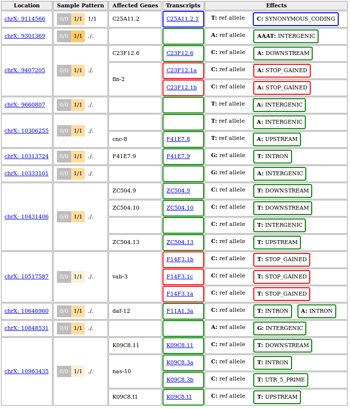
A full-featured report would look like this:

Disclaimer

1. The above output is based on WS220 coordinates (SnpEff v3.6 was installed on our system). If you chose to rebase to WBcel235 before performing the variant annotation, the variant positions in your output should be different. If things worked correctly, the annotated genes, transcripts and effects should be identical though.

2. To get a more compact report we restricted the upstream/downstream interval length for SnpEff-based annotations to 500 bp by running the annotate tool with --ud 500. This turns the effect of variants further than 500bp away from the next gene into type intergenic instead of them getting listed as upstream or downstream of every single isoform of the neighbouring gene.

   This is just one of several possible ways to fine-tune the process of variant annotation. The Variant Annotation tool in Galaxy offers these modifying options in the section More SnpEff options.

The variant at 10,517,587 on chromosome X represents the known ot266 allele. As reported it causes a premature stop codon in three different transcripts known to be generated from the gene vab-3.

Of note, the other nonsense mutation reported in the candidate region at 9,407,205 has also been confirmed experimentally, but was shown not to be responsible for the DAT-1 misexpression phenotype.

Hint

Even in the age of WGS and with the best mapping software (which, of course, you are using when you read this), you have to expect to end up with more than one candidate mutation in a mapped interval.

Typical mutagenesis protocols introduce not just one, but many mutations in a single genome and if a background mutation lies close to your causative mutation it is entirely possible that the two show perfect cosegregation in the limited number of F2 recombinants that you pool for your analysis.

This is a limitation imposed by genetics, which cannot be overcome by any downstream data processing, so always be prepared for follow-up wet lab experiments to confirm or rule out candidate mutations!

End of the Tutorial

Congratulations! You have completed our tutorial and should now have a solid understanding of the basic functionality of most MiModD tools.

As further reading, we suggest

• the Tool Documentation, which has all the details about every parameter that you can use with the different MiModD tools and of which we highlighted just the most important ones in the tutorial, or
• the chapter on Mapping-by-sequencing, which discusses various common mapping strategies for identifying causative mutations and how they can be implemented with MiModD. This should be a good read for you, if after following this third example analysis above, you have the feeling that the type of experiment you would like to analyze with MiModD is not quite like the example.

Besides, all that is left to do for us is to wish you lots of success with your own analyses!