Multi-sample analysis: three-sample analysis of yeast mutants and their parent strain

Background

Wild-type laboratory strains of Saccharomyces cerevisiae, like the reference strain S288C or the widely used strain CEN.PK113-7D, can grow on a variety of carbon sources including lactate.

In a recent publication [2], a knock-out mutant strain based on CEN.PK113-7D was generated, in which the gene for the only known lactate transporter in yeast, JEN1, is disrupted by an inserted reporter cassette. As expected, this strain cannot use lactate as a carbon source. Laboratory evolution was used then on this strain to obtain two substrains that had regained the ability to grow on lactate. Both substrains, IMW004 and IMW005, were subjected to WGS to gain insight into the genomic changes that these strains had undergone compared to CEN.PK113-7D over ~100 generations of laboratory evolution and that might explain their ability to grow on lactate despite the disruption of the JEN1 gene.

Strikingly, the substrains harbored independent point mutations in the acetate transporter gene ADY2 and subsequent experiments showed that these mutations are likely to cause changes in the substrate specificity of this transporter.

This example uses MiModD to recapitulate the primary finding from the laboratory evolution experiment. It will demonstrate how MiModD enables the simultaneous analysis of several samples in a few simple steps, and how the data exploration and annotation tools can be used to narrow down large lists of variants and affected genes efficiently.

The yeastADY2.tar.gz archive available from the MiModD download site contains the following files:

• the S288C reference sequence in fasta format,
• a BAM file of NGS reads from the CEN.PK113-7D parent strain (the reads are a random subset of those available through the NCBI small reads archive (SRA) under accession number SRX129922),
• a BAM file of NGS reads from the lab-evolved substrain IMW004 (the same reads as available under the NCBI SRA accession number SRX129995), and
• a BAM file of NGS reads from the lab-evolved substrain IMW005 (the same reads as available under the NCBI SRA accession number SRX129996).

[2]	(1, 2) Kok et al. (2012): Laboratory evolution of new lactate transporter genes in a jen1D mutant of Saccharomyces cerevisiae and their identification as ADY2 alleles by whole-genome resequencing and transcriptome analysis. FEMS Yeast Res, 12:359-74.

Step 0: Preparing the data

Data preparation for Galaxy

If you are using MiModD through its Galaxy interface, you need to upload the reference fasta and the BAM files of WGS reads to Galaxy just as in the first example. Once the uploads are finished you can proceed to Step 1.

Data preparation for the command line

Apart from extracting the data files from the downloaded archive no special data preparation is required when working from the command line.

As in the first example, we will assume though that you have set your current working directory to the extracted directory, tutorial_ex2. Although this is not an absolute requirement, it will allow you to execute the command line instructions in this section by simply copying/pasting them from this page into a terminal window.

Step 1: Multi-sample NGS Reads Alignment with the MiModD snap tool

Alignments for multiple samples are almost as simple to perform with MiModD as alignments for a single sample.

In Galaxy, start by selecting the reference genome (1) and the first sequenced reads input file (2). Make sure you select BAM as the input format and paired-end as the mode since all WGS data in this example was obtained using Illumina paired-end sequencing.

As before, you do not have to select a custom header file since all BAM files in this example have appropriate header information already. Once you have configured the settings for the first input file, simply add the additional input datasets. You can do this by clicking on the Insert datasets button (3).

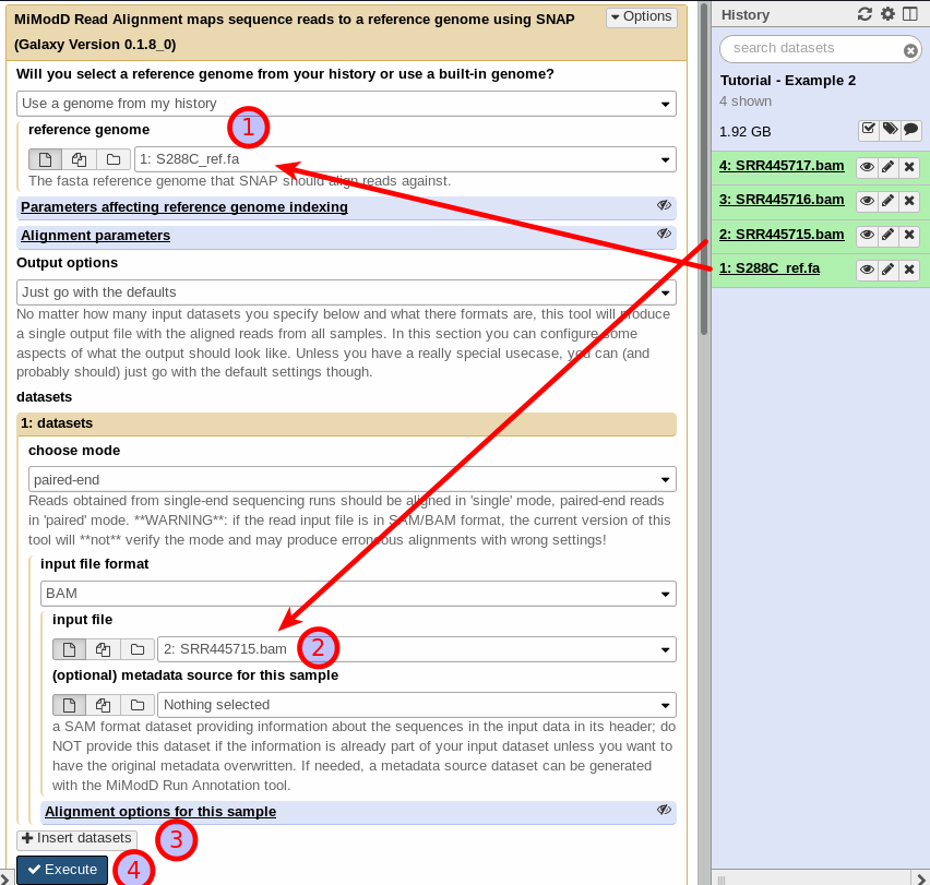
Again, make sure you select the appropriate mode (paired-end) and file format (BAM) for each dataset.

Leave all other settings at their defaults and click on Execute to start your multisample alignment job (4), which will add a single results dataset with the merged alignments of all samples to your history.

If you are using MiModD from the command line, you will have to use the snap-batch tool to align reads from multiple input files. To this tool you have to pass a full valid snap tool call per input file, either as a series of literal commands or as a text file, in which the individual commands are stored on separate lines.

If this sounds complicated, consider this example:

To perform the alignment for just one input file you would issue the following command as we have seen in the First Steps example , e.g.:

mimodd snap paired S288C_ref.fa SRR445715.bam -o SRR445715.aln.bam --verbose

The command line to execute snap-batch for an alignment of all three BAM input files with the same settings as above then takes the following form:

mimodd snap-batch -s "snap paired S288C_ref.fa SRR445715.bam -o example2.aln.bam --verbose" "snap paired S288C_ref.fa SRR445716.bam -o example2.aln.bam --verbose" "snap paired S288C_ref.fa SRR445717.bam -o example2.aln.bam --verbose"

Here, the -s switch indicates that the individual snap calls are specified directly on the command line. Note that the quotes around the individual snap calls are necessary to group the calls (or the shell would split arguments on every whitespace).

Alternatively, you can generate a batch text file (using any editor that lets you store or export plain text) with the following content:

snap paired S288C_ref.fa SRR445715.bam -o example2.aln.bam --verbose
snap paired S288C_ref.fa SRR445716.bam -o example2.aln.bam --verbose
snap paired S288C_ref.fa SRR445717.bam -o example2.aln.bam --verbose

and then call snap-batch like this (the -f switch tells the tool to read the snap commands from the specified file):

mimodd snap-batch -f <batch file>

Note

In both versions of the snap-batch command you need to provide the -o switch with every single snap command just to form a valid call. Since snap-batch will always produce just a single merged output, it takes the output file name from the first snap command that is provided and ignores additional output file specifications in later commands.

See also

the snap-batch tool description in the Tool Documentation.

Step 2: Identification of Sequence Variants from a multi-sample alignment

Variant calling from a multi-sample alignment as input is really no different from the single-sample procedure illustrated in the first example.

MiModD will correctly identify read groups and samples present in the input file of aligned reads and handle them appropriately.

We leave it up to you to run this very simple job from Galaxy, but here is the command line equivalent to copy/paste:

mimodd varcall S288C_ref.fa example2.aln.bam -o example2_calls.bcf --verbose

More on multisample alignment and variant calling

• Multisample alignment is mostly for your convenience: we think it is easier to handle a single aligned reads dataset/file than several, but the alignment result will be the same no matter whether it is generated through one multisample or through several single sample alignment jobs.

  If you prefer to have individual alignment results for each of your input datasets, there is nothing wrong with that. In fact, the Variant Calling/varcall tool accepts multiple aligned reads datasets/files as input so you can still combine your data into one bcf output of variant call information.

• Multisample variant calling, on the other hand, produces different results than multiple single-sample analyses.

  A multisample analysis can employ statistical methods to borrow information between samples that are not available during separate single-sample analyses. This allows a multisample analysis to detect shared variants, that occur in several samples, with higher sensitivity.

  In addition, variants extracted from multisample bcf data will have associated statistical information about sites that are variant in any of the samples, i.e. the output will not only contain information about why the variant was called in a given sample, but also why and how reliably it was not called in others.

  For these reasons, all downstream tools in MiModD are designed to operate on multisample variant lists as their input and you are strongly encouraged to combine the data from all samples that you sequenced to answer a given biological question at the variant calling stage.

Step 3: Identification of Deletions

Like for Variant Calling, there is no difference between the Deletion Calling step for single-sample and multi-sample input.

Again, MiModD will auto-detect all read groups and samples in the input file and handle them appropriately. The result is a single output file, in which deletions (and possibly uncovered regions) are reported along with the sample in which they were detected.

From the command line you can use delcall with:

mimodd delcall example2.aln.bam example2_calls.bcf -o example2_deletions.txt --max-cov 4 --min-size 100

Step 4: Data Exploration and Annotation

The real difference between a single-sample WGS analysis and the analysis of multiple samples lies in the complexity of the biological questions that can be addressed with multisample data.

Possible questions in this example are:

1. What differences exist between the parent strain of the study, CEN.PK113-7D, and the reference strain S288C?
2. What differences exist between the evolved strain IMW004 and its parent CEN.PK113-7D?
3. What differences exist between the second evolved strain IMW005 and its parent CEN.PK113-7D?
4. Are there common effects of these differences in IMW004 and IMW005?

Note that the first question is only of secondary interest here compared to the second and the third, but most importantly, that the naive question

What differences exist between each of the evolved strains and the reference ?

is not very helpful since the set of these differences will be the union of the differences between CEN.PK113-7D and S288C and the differences between each evolved strain and CEN.PK113-7D. In fact, this is the reason why it is essential to include sequencing data for CEN.PK113-7D in the analysis.

Also note that the fourth question is not about shared differences in IMW004 and IMW005. Since these two strains have evolved completely separately, the chance of them sharing an exactly identical variation that is not present in their parent strain is extremely low. However, it is certainly possible that different variants in the two strains will affect the same genomic feature (e.g., the same gene), which could then be taken as evidence that this gene may be of importance for the observed biological effect (growth on lactate in this case).

Extracting the combined variant pool

Before we can answer any of our questions though, we need to extract the total set of variants detected at the variant calling step. From the command line this is done through:

mimodd varextract example2_calls.bcf -o example2_extracted_variants.vcf

Again, we leave it up to you to do the same from Galaxy.

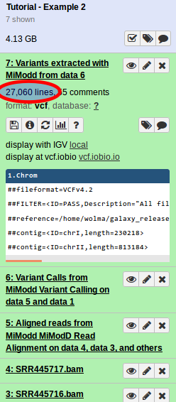
A quick look at the results reveals that, in total, over 27000 (!) variants (SNVs and indels) have been detected (see figure on the left).

These include differences between any of the three sequenced samples and the reference genome along with false-positive calls. The goal of this analysis step is to filter and annotate this impressive list in different ways to remove false-positive variants and to retain only those that help us answer the four questions defined above.

This section demonstrates how the vcf-filter, annotate and varreport tools can be used together for this purpose.

Note

In principle, deletions predicted in the Deletion Calling step should be treated the same way, preferably together with the other variants. The current version of MiModD, however, does not offer any tools to post-process the deletion output file. Luckily, the number of predicted deletions is typically much smaller than that of other variants, so inspecting the full list of deletions is possible (though, admittedly, inconvenient).

Q1: Differences between the parent strain of the study, CEN.PK113-7D, and the reference strain S288C

The key to answering most of our questions is to use the vcf-filter tool with appropriate sample-specific filters.

A simple filter corresponding to question 1 can be formulated on the command line as:

mimodd vcf-filter example2_extracted_variants.vcf -o example2_q1_filter1_variants.vcf -s CEN.PK113-7D --gt 1/1,0/1 --dp 0 --gq 0

, which reports all variants for which the CEN.PK113-7D sample appears to be heterozygous or homozygous mutant. With this approach we get rid of more than 1000 variants, but are still left with over 25000.

It is quite easy, however, to make the filter more stringent, e.g., we can try:

mimodd vcf-filter example2_extracted_variants.vcf -o example2_q1_filter2_variants.vcf -s CEN.PK113-7D --gt 1/1,0/1 --dp 3 --gq 0

, which is very similar to the first version but, in addition, is asking for at least three fold coverage of the variant for the CEN.PK113-7D sample. Adding this new criterium, leaves us with just below 25000 variants.

CEN.PK113-7D is a haploid yeast strain and heterozygous calls are likely indicating sites at which variant calling is unreliable, so there is justification (as discussed for the first example) for using:

mimodd vcf-filter example2_extracted_variants.vcf -o example2_q1_filter3_variants.vcf -s CEN.PK113-7D --gt 1/1 --dp 3 --gq 0

to retain only homozygous variants, which turn out to be ~ 23500 in our case.

Finally, we could reason that true sequence deviations between CEN.PK113-7D and the reference strain S288C are very likely to occur also in the derived strains IMW004 and IMW005. Thus, we can add additional filters for these samples resulting in:

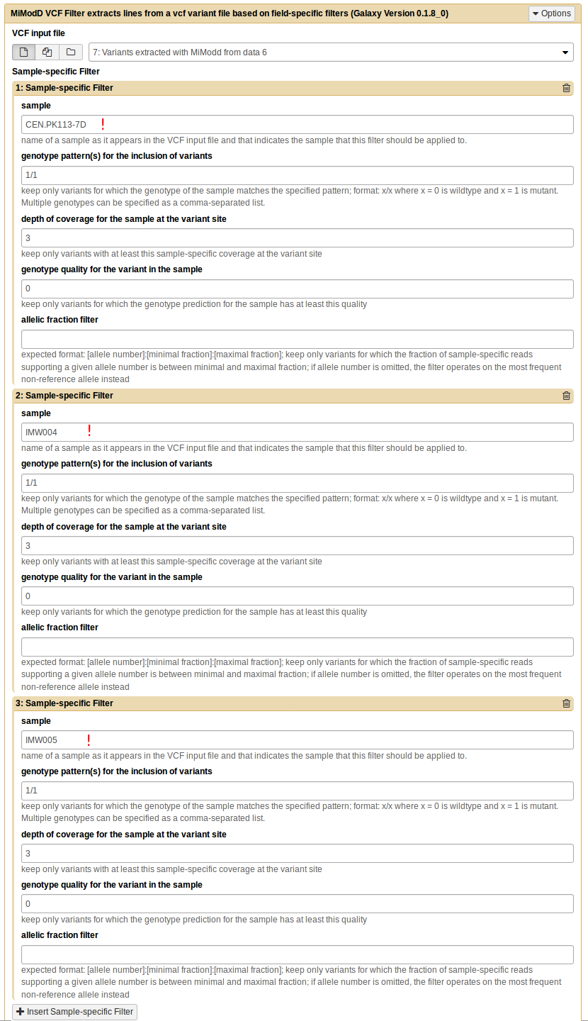
mimodd vcf-filter example2_extracted_variants.vcf -o example2_q1_filter4_variants.vcf -s CEN.PK113-7D IMW004 IMW005 --gt 1/1 1/1 1/1 --dp 3 3 3 --gq 0 0 0

, which only retains variants for which all three sequenced samples appear to be homozygous mutant and for which there is an at least 3-fold coverage in all three samples. Applying this filter gives us a list of ~ 22500 variants representing our best candidates for true variant sites between S288C and CEN.PK113-7D.

To compose this last job from Galaxy, open the VCF Filter tool, select the VCF input file, then define the three sample-specific filters (add them by clicking on Insert Sample-specific Filter) shown below:

Q2: Differences between the evolved strain IMW004 and its parent CEN.PK113-7D

Here we are looking for variants in IMW004 that are not present in the parent strain CEN.PK113-7D. To get them we can use:

mimodd vcf-filter example2_extracted_variants.vcf -o example2_q2_variants.vcf -s CEN.PK113-7D IMW004 IMW005 --gt 0/0 1/1 0/0 --dp 3 3 3 --gq 0 0 0

The rationale for including IMW005 in this filter and only accepting variants that are absent from this strain is that the laboratory evolution experiment was not started with CEN.PK113-7D, but with a derived strain genetically engineered to have the JEN1 gene disrupted. The sequence of this strain is not available, and the idea is that variants found in IMW004 and IMW005, but not CEN.PK113-7D, must have first occurred in the unsequenced JEN1delta strain and, thus, were present at the start of the experiment, which makes them less interesting.

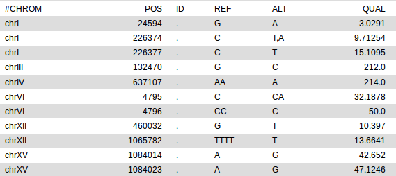
Applying this filter leaves us with only 16 variants (out of the initial 27000)! The list (produced in Galaxy) is shown below.

Q3: Differences between the evolved strain IMW005 and its parent CEN.PK113-7D

This question can, of course, be answered by just slightly modifying our last filter settings to:

mimodd vcf-filter example2_extracted_variants.vcf -o example2_q3_variants.vcf -s CEN.PK113-7D IMW005 IMW004 --gt 0/0 1/1 0/0 --dp 3 3 3 --gq 0 0 0

With the roles of IWM005 and IMW004 reverted, we get the following list of 11 variants:

Q4: Differences with common effects in IMW004 and IMW005

This question, asking for distinct variants in IMW004 and IMW005 that have a common effect on a genomic feature, is the most challenging one.

In this example, with the small number of variants obtained as answers to questions 2 and 3, it is not too difficult to find the two variants - one in IMW004, the other in IMW005 - that are in suspiciously close genomic vicinity, i.e., that may well affect the same gene.

Using the varreport tool though we can make this task a lot easier.

As part of the first example, we have looked at the most basic functionality of the tool, which is to turn a vcf file into a stripped down tabular report file. However, varreport can do more than this.

If you choose HTML as the output format instead of Tab-separated plain text, the tool will try to enrich its output with species-specific hyperlinks if possible.

One type of hyperlink, which you can get with almost no additional effort, lets you explore the surroundings of the genomic positions of your variants in the standard genome browser for your organism of interest.

The current version of MiModD comes with built-in support for generating species-specific hyperlinks for the following seven model organisms:

• the cyanobacterium Synechocystis PCC6803
• baker’s yeast (S. cerevisiae)
• thale cress (A. thaliana)
• the roundworm C. elegans
• the fruitfly D. melanogaster
• zebrafish (D. rerio)
• the ciliate Tetrahymena thermophila

For these species, it is enough to provide varreport with the species name (several aliases are supported) to have the correct genome browser hyperlinks generated.

If you are working with a different species you can provide your own template file with hyperlink formatting instructions.

The second type of hyperlink that varreport can generate is to gene/transcript pages of organism-specific database portals. For this to work, however, you will have to combine the tool with the annotate tool, to add the information about affected genes and transcripts to your VCF variants file first.

Note

Weblinks are changing frequently and it is entirely possible that hyperlinks for your species of interest suddenly stop working. Custom template files offer a solution for this kind of problem until we provide a software update.

If you discover broken hyperlinks or generate a template file that you want to share with a larger community, you should contact us and we will be more than happy to fix the problem or to add your organism to the list of natively supported species.

Enhancing variant reports through genome browser hyperlinks

Generating hyperlinks to genome browser views of genomic regions has no requirements other than a valid hyperlink template or built-in species support. For our example, we can generate an annotated file from Galaxy by configuring the Report Variants tool as shown below (the input file here is the list of IMW005-specific variants generated as answer to Q3):

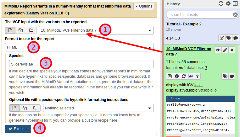
All you have to do is to set the output format to HTML and to provide the species name.

The command line equivalent of this Galaxy job is:

mimodd varreport example2_q3_variants.vcf --species S.cerevisiae -o example2_q3_report.html -f html

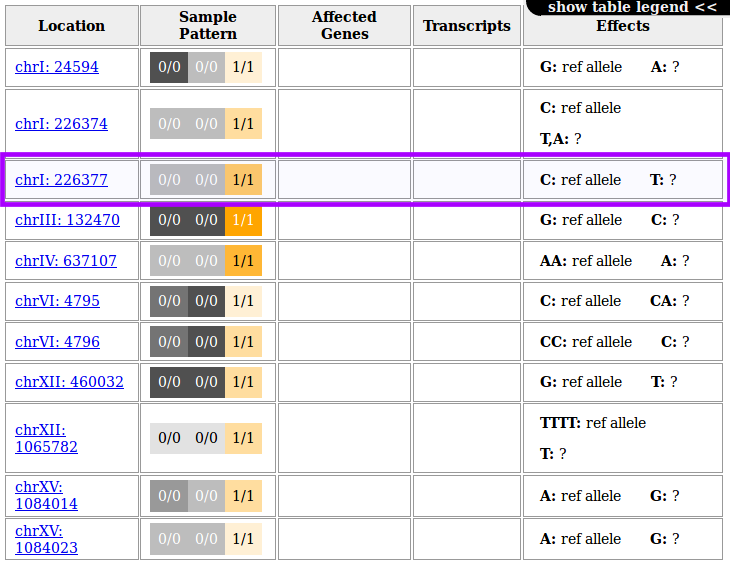
The result of this step is a new dataset the contents of which can be viewed in any web browser. If you performed this step in Galaxy, viewing the result requires two steps: first, click on the dataset’s eye symbol, then follow the link that gets displayed and takes you to the results page.

It should look like this:

Hint

If instead you are greeted with

This page will look so much nicer when it’s styled!

If you are viewing this through Galaxy, then the Galaxy server is blocking the style information accompanying the page. In this case, we recommend you to:

1. download the dataset,
2. extract the variant_report.html file from the resulting zip archive and
3. open this local file with your browser.

, then the Galaxy you are using prevents html content from displaying with its style information applied. You can then either follow the above instructions or ask the administrator of the Galaxy instance you are working on to whitelist the MiModD Report Variants tool as a safe tool, html output of which can be displayed without restrictions. If you are the administrator, here is a how to do this yourself.

Following any of the position links will take you to the yeastgenome.org genome browser and will zoom in on a 1kb region around the variant site.

For the highlighted variant, for example, this would look like this:

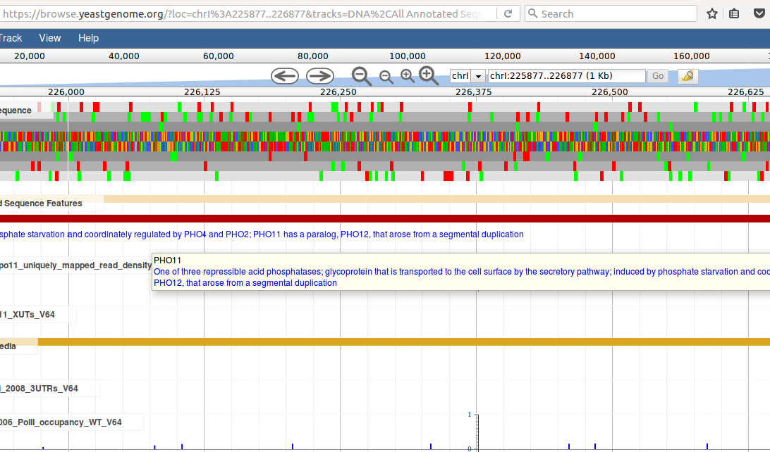
quickly showing that this variant lies in the gene PHO11.

Warning

If the version of the reference genome you are using is different from that used by the genome browser, the simple 1:1 mapping between variant sites reported by MiModD and positions shown in the genome browser may be inaccurate !

Make sure you are using a compatible genome version for your organism and do not rely on the genome browser view alone to determine the exact location of variations !

Including effects on genomic features in variant reports

To annotate variants with their effects on genomic features, such as transcripts and genes, MiModD relies on SnpEff - a toolbox for genetic variant annotation and effect prediction.

The MiModD installation instructions have a separate section on the installation and inital setup of SnpEff.

If you have configured MiModD to use SnpEff and you have a SnpEff genome file for yeast installed (genome file EF3.64 is assumed here), you can obtain a new VCF variants file annotated with the effects of the variants on genes and transcripts via the following command line:

mimodd annotate example2_q3_variants.vcf EF3.64 -o example2_q3_anno.vcf

, where the SnpEff genome file gets passed right after the VCF input file.

Hint

The genome file name could be different for your installation (e.g., if you chose to download a different version).

The example above assumes the SnpEff 3.6 genome file EF3.64, but in SnpEff v4.x the equivalent genome is called R64-1-1.xx, where xx is a frequently changing sub-version number. We will have a much more detailed look at SnpEff genome versions in the third example analysis of this tutorial.

If you do not know or do not remember the name of the genome file you can use the simple snpeff-genomes tool like this:

mimodd snpeff-genomes

to get a list of all currently installed SnpEff genome files on your system together with organism names.

From within Galaxy you can run the List Installed SnpEff Genomes tool, which will produce a tabular text dataset with the same information.

When viewed directly, the annotated VCF may not appear very helpful, but with it as input, the varreport tool can do a better job and provide us with a fully featured report. Running:

mimodd varreport example2_q3_anno.vcf -o example2_q3_report.html -f html

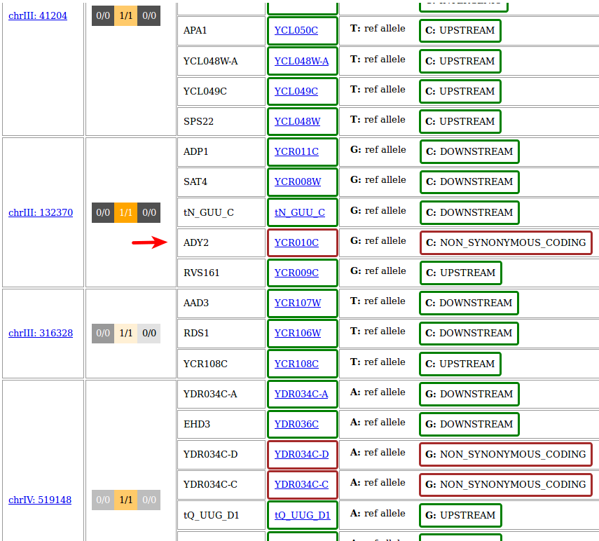
now gives this output:

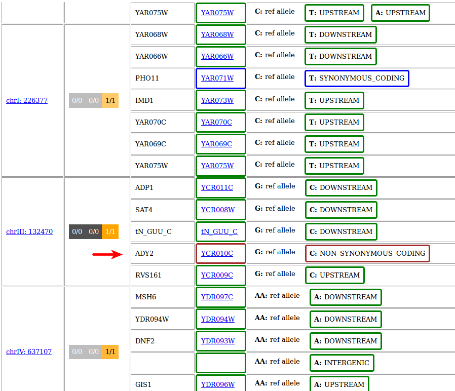
In it, all effects of every input variant on any genomic feature described in the SnpEff genome file are reported, and it is now very easy to see that the only variant with a direct effect at the protein level is in the gene ADY2.

Apart from this spectacular success :), note that, compared to the command in the previous section, we did not have to provide the species information anymore. This is because the annotate tool, which knew about the species, stored this information in its output and varreport picks it up again.

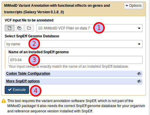
Running the same job from Galaxy is straightforward if you know the name of the SnpEff genome that you want to use. Using the MiModD Variant Annotation tool, you select the original vcf dataset that you would like to annotate (1), then choose Select Snpeff Genome Database by name (2). In the example shown below we are then using EF3.64 just like in the command line call and run the job (4).

The resulting dataset can be used as input to the Report Variants tool, which should then produce the same output as shown for the command line call. Just as in the command line example, again, you will not have to set the Species explicitly to use the tool because that information is already recorded in the input dataset.

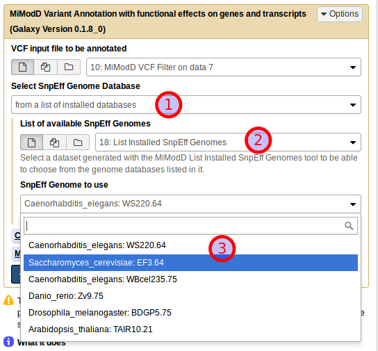
If you do not know the name of the SnpEff genome, but you have run the List Installed SnpEff Genomes tool before, you can, instead, select the SnpEff genome database from a list of installed databases (1), then choose the dataset generated by that tool as your List of available SnpEff Genomes (2) and select the right genome from a dropdown list of available choices (3).

As an exercise you can now try to annotate and report the IMW004-specific variants!

The result should look like this and reveal that, just as expected, ADY2 is affected by a non-synonymous mutation also in this sample.

Note the position of the variant, which is different from that in the previous result, showing that IMW004 and IMW005 really carry two different mutations (though both happen to be G->C transversions in ADY2).

Finally, if you want to learn more about ADY2 to understand how a mutation in it can possibly substitute for the lost lactate transporter JEN1, you can follow the YCR010C transcript link right next to it in any of the two variant reports and you should be taken to the corresponding gene page of the Saccharomyces Genome Database:

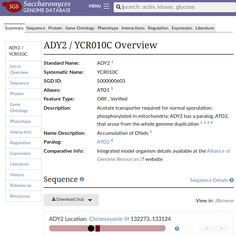
Et voilà, the gene encodes a transporter for acetate, which the authors of our paper [2] find to change substrate specificity when affected by either of the two mutations.

End of Part 2 of the Tutorial

In this part you have learnt how you can combine several of MiModD’s data exploration tools to identify causative variants through comparison of several samples. Importantly, however, the analysis above did not rely on crosses between any strains, but only on shared ancestry. If you are interested in identifying causative variants following mapping crosses, be sure to continue with the next section.